How to Make a Time Series Plot with Rolling Average in Python?
Last Updated :
02 Dec, 2020
Time Series Plot is used to observe various trends in the dataset over a period of time. In such problems, the data is ordered by time and can fluctuate by the unit of time considered in the dataset (day, month, seconds, hours, etc.). When plotting the time series data, these fluctuations may prevent us to clearly gain insights about the peaks and troughs in the plot. So to clearly get value from the data, we use the rolling average concept to make the time series plot.
The rolling average or moving average is the simple mean of the last ‘n’ values. It can help us in finding trends that would be otherwise hard to detect. Also, they can be used to determine long-term trends. You can simply calculate the rolling average by summing up the previous ‘n’ values and dividing them by ‘n’ itself. But for this, the first (n-1) values of the rolling average would be Nan.
In this article, we will learn how to make a time series plot with a rolling average in Python using Pandas and Seaborn libraries. Below is the syntax for computing rolling average using pandas.
Syntax: pandas.DataFrame.rolling(n).mean()
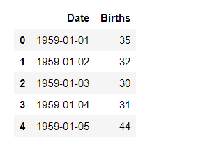
We will be using the ‘Daily Female Births Dataset’. This dataset describes the number of daily female births in California in 1959. There are 365 observations from 01-01-1959 to 31-12-1959. You can download the dataset from this link.
Let’s Implement with step-wise:
Step 1: Import the libraries.
Python3
import pandas as pd
import seaborn as sns
import matplotlib.pyplot as plt
|
Step 2: Import the dataset
Python3
data = pd.read_csv( "https://raw.githubusercontent.com/jbrownlee/ \
Datasets/master/daily-total-female-births.csv")
display( data.head())
|
Output:
Step 3: Plot a simple time series plot using seaborn.lineplot()
Python3
plt.figure( figsize = ( 12, 5))
sns.lineplot( x = 'Date',
y = 'Births',
data = data,
label = 'DailyBirths')
plt.xlabel( 'Months of the year 1959')
pos = [ '1959-01-01', '1959-02-01', '1959-03-01', '1959-04-01',
'1959-05-01', '1959-06-01', '1959-07-01', '1959-08-01',
'1959-09-01', '1959-10-01', '1959-11-01', '1959-12-01']
lab = [ 'Jan', 'Feb', 'Mar', 'Apr', 'May', 'June',
'July', 'Aug', 'Sept', 'Oct', 'Nov', 'Dec']
plt.xticks( pos, lab)
plt.ylabel('Female Births')
|
Output:
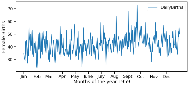
We can notice that it is very difficult to gain knowledge from the above plot as the data fluctuates a lot. So, let us plot it again but using the Rolling Average concept this time.
Step 4: Compute Rolling Average using pandas.DataFrame.rolling.mean().
For rolling average, we have to take a certain window size. Here, we have taken the window size = 7 i.e. rolling average of 7 days or 1 week.
Python3
data[ '7day_rolling_avg' ] = data.Births.rolling( 7).mean()
Display(data.head(10))
|
Output:
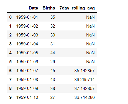
We can observe that the first 6 values of the ‘7day_rolling_avg’ column are NaN values. This is because these 6 values don’t have enough data to compute the rolling average of 7 days. So, in the plot also, for the first six values, no values would be plotted.
Step 5: Make a time series plot using rolling average calculated in step 4
Python3
plt.figure( figsize = ( 12, 5))
sns.lineplot( x = 'Date',
y = 'Births',
data = data,
label = 'DailyBirths')
sns.lineplot( x = 'Date',
y = '7day_rolling_avg',
data = data,
label = 'Rollingavg')
plt.xlabel('Months of the year 1959')
pos = [ '1959-01-01', '1959-02-01', '1959-03-01', '1959-04-01',
'1959-05-01', '1959-06-01', '1959-07-01', '1959-08-01',
'1959-09-01', '1959-10-01', '1959-11-01', '1959-12-01']
lab = [ 'Jan', 'Feb', 'Mar', 'Apr', 'May', 'June',
'July', 'Aug', 'Sept', 'Oct', 'Nov', 'Dec']
plt.xticks( pos, lab)
plt.ylabel('Female Births')
|
Output:

We can clearly see through the above graph that the rolling average has smoothened the number of female births, and we can notice the peak more evidently.
Share your thoughts in the comments
Please Login to comment...