Measures of Dispersion are used to represent the scattering of data. These are the numbers that show the various aspects of the data spread across various parameters.
Let’s learn about the measure of dispersion in statistics , its types, formulas, and examples in detail.
Dispersion in Statistics
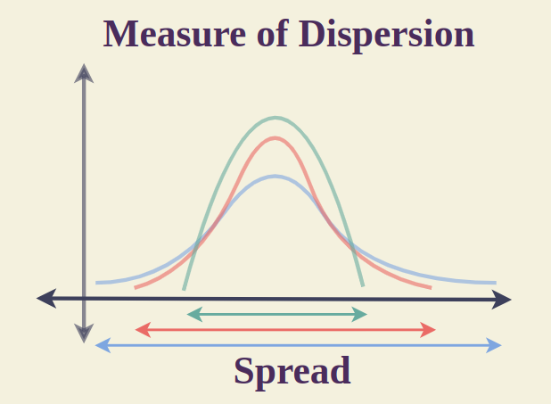
Dispersion in statistics is a way to describe how spread out or scattered the data is around an average value. It helps to understand if the data points are close together or far apart.
Dispersion shows the variability or consistency in a set of data. There are different measures of dispersion like range, variance, and standard deviation.
Measure of Dispersion in Statistics
Measures of Dispersion measure the scattering of the data. It tells us how the values are distributed in the data set. In statistics, we define the measure of dispersion as various parameters that are used to define the various attributes of the data.
These measures of dispersion capture variation between different values of the data.
Types of Measures of Dispersion
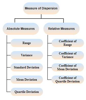
Measures of dispersion can be classified into the following two types :
- Absolute Measure of Dispersion
- Relative Measure of Dispersion
These measures of dispersion can be further divided into various categories. They have various parameters and these parameters have the same unit.
Let’s learn about them in detail.
Absolute Measure of Dispersion
The measures of dispersion that are measured and expressed in the units of data themselves are called Absolute Measure of Dispersion. For example – Meters, Dollars, Kg, etc.
Some absolute measures of dispersion are:
Range: It is defined as the difference between the largest and the smallest value in the distribution.
Mean Deviation: It is the arithmetic mean of the difference between the values and their mean.
Standard Deviation: It is the square root of the arithmetic average of the square of the deviations measured from the mean.
Variance: It is defined as the average of the square deviation from the mean of the given data set.
Quartile Deviation: It is defined as half of the difference between the third quartile and the first quartile in a given data set.
Interquartile Range: The difference between upper(Q3 ) and lower(Q1) quartile is called Interterquartile Range. Its formula is given as Q3 – Q1.
Read More :
Relative Measure of Dispersion
We use relative measures of dispersion to measure the two quantities that have different units to get a better idea about the scattering of the data.
Here are some of the relative measures of dispersion:
Coefficient of Range: It is defined as the ratio of the difference between the highest and lowest value in a data set to the sum of the highest and lowest value.
Coefficient of Variation: It is defined as the ratio of the standard deviation to the mean of the data set. We use percentages to express the coefficient of variation.
Coefficient of Mean Deviation: It is defined as the ratio of the mean deviation to the value of the central point of the data set.
Coefficient of Quartile Deviation: It is defined as the ratio of the difference between the third quartile and the first quartile to the sum of the third and first quartiles.
Read More :
Range of Data Set
The range is the difference between the largest and the smallest values in the distribution.
Thus, it can be written as
R = L – S
where,
L is the largest value in the Distribution
S is the smallest value in the Distribution
- A higher value of range implies higher variation in the data set.
- One drawback of this measure is that it only takes into account the maximum and the minimum value. They might not always be the proper indicator of how the values of the distribution are scattered.
Example: Find the range of the data set 10, 20, 15, 0, 100.
Solution:
- Smallest Value in the data = 0
- Largest Value in the data = 100
Thus, the range of the data set is,
R = 100 – 0
R = 100
Note: Range cannot be calculated for the open-ended frequency distributions. Open-ended frequency distributions are those distributions in which either the lower limit of the lowest class or the higher limit of the highest class is not defined.
Range for Ungrouped Data
To find the range for the ungrouped data set, first we have to find the smallest and the largest value of the data set by observing. The difference between them gives the range of ungrouped data.
We can understyand this with the help of following example:
Example: Find out the range for the following observations, 20, 24, 31, 17, 45, 39, 51, 61.
Solution:
- Largest Value = 61
- Smallest Value = 17
Thus, the range of the data set is
Range = 61 – 17 = 44
Range for Grouped Data
The range of the grouped data set is found by studying the following example,
Example: Find out the range for the following frequency distribution table for the marks scored by class 10 students.
Solution:
- For Largest Value: Taking the higher limit of Highest Class = 40
- For Smallest Value: Taking the lower limit of Lowest Class = 0
Range = 40 – 0
Thus, the range of the given data set is,
Range = 40
Mean Deviation
Mean deviation measures the deviation of the observations from the mean of the distribution.
Since the average is the central value of the data, some deviations might be positive and some might be negative. If they are added like that, their sum will not reveal much as they tend to cancel each other’s effect.
For example :
Let us consider this set of data : -5, 10, 25
Mean = (-5 + 10 + 25)/3 = 10
Now a deviation from the mean for different values is,
- (-5 -10) = -15
- (10 – 10) = 0
- (25 – 10) = 15
Now adding the deviations, shows that there is zero deviation from the mean which is incorrect. Thus, to counter this problem only the absolute values of the difference are taken while calculating the mean deviation.
Mean Deviation Formula :
MD = 
Mean Deviation for Ungrouped Data
For calculating the mean deviation for ungrouped data, the following steps must be followed:
Step 1: Calculate the arithmetic mean for all the values of the dataset.
Step 2: Calculate the difference between each value of the dataset and the mean. Only absolute values of the differences will be considered. |d|
Step 3: Calculate the arithmetic mean of these deviations using the formula,
M.D = 
This can be explained using the example.
Example: Calculate the mean deviation for the given ungrouped data, 2, 4, 6, 8, 10
Solution:
Mean(μ) = (2+4+6+8+10)/(5)
μ = 6
M. D =
⇒ M.D = 
⇒ M.D = (4+2+0+2+4)/(5)
⇒ M.D = 12/5 = 2.4
Read More On :
Measures of Dispersion Formulas are used to tell us about the various parameters of the data. Various formulas related to the measures of dispersion are discussed in the table below.
|
Formulae of Measures of Dispersion
|
| Range | H – S
where, H is the Largest Value and S is the Smallest Value
|
| Variance | Population Variance, σ2 = Σ(xi-μ)2 /n
Sample Variance, S2 = Σ(xi-μ)2 /(n-1)
where, μ is the mean and n is the number of observation
|
| Standard Deviation | S.D. = √(σ2) |
| Mean Deviation | μ = (x – a)/n
where, a is the central value(mean, median, mode) and n is the number of observation
|
| Quartile Deviation | (Q3 – Q1)/2
where,Q3 = Third Quartile and Q1 = First Quartile
|
Coefficient of Dispersion
Coefficients of dispersion are calculated when two series are compared, which have great differences in their average. We also use co-efficient of dispersion for comparing two series that have different measurements. It is denoted using the letters C.D.
|
| Coefficient of Range | (H – S)/(H + S) |
| Coefficient of Variation | (SD/Mean)×100 |
| Coefficient of Mean Deviation | (Mean Deviation)/μ
where,
μ is the central point for which the mean is calculated
|
| Coefficient of Quartile Deviation | (Q3 – Q1)/(Q3 + Q1) |
Measures of Dispersion and Central Tendency
Both Measures of Dispersion and Central Tendency are numbers that are used to describe various parameters of the data. Let’s see the differences between Measures of Dispersion and Central Tendency.
|
Central Tendency vs. Measure of Dispersion
|
Central Tendency is a term used for the numbers that quantify the properties of the data set.
| Measure of Distribution is used to quantify the variability of the data of dispersion.
|
Measure of Central tendency include,
| Various parameters included for the measure of dispersion are,
- Range
- Variance
- Standard Deviation
- Mean Deviation
- Quartile Deviation
|
Related :
Examples on Measures of Dispersion
Let’s solve some questions on the Measures of Dispersion.
Examples 1: Find out the range for the following observations. {20, 42, 13, 71, 54, 93, 15, 16}
Solution:
Given,
- Largest Value of Observation = 71
- Smallest Value of Observation = 13
Thus, the range of the data set is,
Range = 71 – 13
Range = 58
Example 2: Find out the range for the following frequency distribution table for the marks scored by class 10 students.
Solution:
Given,
- Largest Value: Take the Higher Limit of the Highest Class = 40
- Smallest Value: Take the Lower Limit of the Lowest Class = 10
Range = 40 – 10
Range = 30
Thus, the range of the data set is 30.
Example 3: Calculate the mean deviation for the given ungrouped data {-5, -4, 0, 4, 5}
Solution:
Mean(μ) = {(-5)+(-4)+(0)+(4)+(5)}/5
μ = 0/5 = 0
M. D =
⇒ M.D = 
⇒ M.D = (5+4+0+4+5)/5
⇒ M.D = 18/5
⇒ M.D = 3.6
Measures of Dispersion- FAQs
What is Measure of Dispersion in Statistics?
Measure of Dispersion is the positive real numbers that are used to define the variability of the data set about any central point.
What are Types of Measures of Dispersion in Statistics?
Measures of Dispersion are classified into two types :
- Absolute Measures of Dispersion
- Relative Measures of Dispersion
What is Absolute Measure of Dispersion?
Absolute Measures of Dispersion are the statistical tools that provide the actual spread of data, like range and standard deviation. They have the same units as the data.
What is Relative Measure of Dispersion?
Relative Measure of Dispersions show the spread of data relative to its central value, without unit dependency. They are statistical comparisons, expressed as ratios or percentages, like the coefficient of variation.
What is the Difference between Absolute and Relative Measure of Dispersion?
Absolute measures of dispersion provide the actual spread of data, like range, variance, standard deviation. They are expressed in the same units as the data. Relative measures of dispersion, on the other hand, compare the spread relative to the central value, usually as a ratio or percentage. They are unitless, allowing for comparison between different datasets.
How to Calculate Dispersion in Statistics?
Dispersion is calculated by using various formulas for mean, standard deviation, variance, etc.
What are Examples of Dispersion in Statistics?
Examples of dispersion in statistics include: Range, Variance, Standard Deviation, Interquartile Range (IQR), Coefficient of Variation, etc.
Share your thoughts in the comments
Please Login to comment...