GeeksforGeeks come forward to reduce the pressure on a student for collecting all the important formulas used in their Class 8 curriculum in a single place. GeeksforGeeks’s Class 8 Maths Formulas are developed in such a way that it covers all the important formulas and properties used in each and every chapter, all in brief. This helps a student to revise and learn easily and quickly. For a Class 8 student, the increase in difficulty level from one’s prior classes might be tough to grasp. In addition, with a discipline like Mathematics, you must remain aware at all times. The subject is quite important in both your schooling and your personal life. To get a high level of knowledge, you must first master your Maths Formulas for Class 8 before moving on to applying them to your questions.
You might be wondering where you can obtain the exact Maths formulas for Class 8 for a certain set of questions. This is why GeeksforGeeks is putting this information in front of you right now. Below mentioned are all of the Maths formulas for Class 8 on one page for you so you don’t have to look for another!
Chapter 1: Rational Numbers
In arithmetic, the different sorts of numbers include integers, real numbers, natural numbers, whole numbers, fractional numbers, prime numbers, and composite numbers. The different types of rational numbers are covered in the Rational Numbers Class 8 math formulae, which will help students learn the concepts of rational numbers, their uniqueness from the rest of the numbers, and their use in higher arithmetic.
Any number that may be expressed as a ⁄ b where b ≠ 0 are rational numbers. The following are the formulas and properties used for rational numbers:
- Additive Identity: (a ⁄ b + 0) = (a ⁄ b).
- Multiplicative Identity: (a ⁄ b) × 1 = (a/b).
- Multiplicative Inverse: (a ⁄ b) × (b/a) = 1.
- Additive Inverse: a + (-a) = (-a) + a = 0.
- Closure Property – Addition: For any two rational numbers a and b, a + b is also a rational number.
- Closure Property – Subtraction: For any two rational numbers a and b, a – b is also a rational number.
- Closure Property – Multiplication: For any two rational numbers a and b, a × b is also a rational number.
- Closure Property – Division: Rational numbers are not closed under division.
- Commutative Property – Addition: For any rational numbers a and b, a + b = b + a.
- Commutative Property – Subtraction: For any rational numbers a and b, a – b ≠ b – a.
- Commutative Property – Multiplication: For any rational numbers a and b, (a x b) = (b x a).
- Commutative Property – Division: For any rational numbers a and b, (a/b) ≠ (b/a).
- Associative Property – Addition: For any rational numbers a, b, and c, (a + b) + c = a + (b + c).
- Associative Property – Subtraction: For any rational numbers a, b, and c, (a – b) – c ≠ a – (b – c)
- Associative Property – Multiplication: For any rational number a, b, and c, (a x b) x c = a x (b x c).
- Associative Property – Division: For any rational numbers a, b, and c, (a / b) / c ≠ a / (b / c).
- Distributive Property: For any three rational numbers a, b and c, a × ( b + c ) = (a × b) +( a × c).
Chapter 2: Linear Equations in One Variable
The linear equation in one variable is an expression that is denoted as ax+b = 0, where a and b are any two integers, and x is a variable and consists of only one solution. As the name suggests linear equation in one variable, the equation of this type has only one solution. There are four different ways to solve Linear equations in one variable:
-
Linear equations of the type that has a Linear expression on one side and numbers on the other side:
- Transpose the number to the side where all numbers are present, maintaining the sign of the number.
- Solve (Add/subtract) the equation on both sides to get it as simpler as possible, to obtain the value of the variable.
-
Linear equations of the type that has variables on both sides:
- Transpose both the number and the variable to get each on the same side maintaining the sign of the number.
- Solve (Add/subtract) the equation on both sides to get it as simpler as possible, to obtain the value of the variable.
-
Linear equations of the type that has a number in the denominator and variables on both sides:
- LCM of the denominator on both sides should be taken
- Then multiply the LCM on both sides so that the equation is deduced to a simple form and then solve it like the Linear equations of the type that has variables on both sides to obtain the value of the variable.
-
Linear equations of the type that are Reducible to the Linear form:
- Such equations are of the form: (x + a / x + b) = c / d.
- Therefore, these equations are solved by the cross-multiplying numerator and denominator to get it into a simple linear form like (x + a) d = c (x + b). This is a Linear equation of the type that has variables on both sides which can be solved further to obtain the value of the variable.
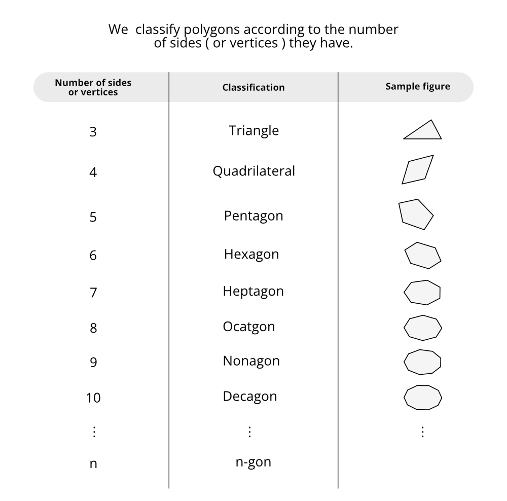
Chapter 3: Understanding Quadrilaterals
A quadrilateral is a closed object with four sides, four vertices, and four angles that is a sort of polygon. It is made up of four non-collinear points that are joined together. The sum of a quadrilateral’s internal angles is always 360 degrees. Lets us now understand the following important notes about the formulae discussed in this chapter:
- Classification of Polygons: The polygons are classified according to the number of sides (or vertices) they have, as mentioned below:
- Angle Sum Property: This property states that the sum of all angles of a quadrilateral is 360°.
- Sum of the Measures of the Exterior Angles of a Polygon: Regardless of the number of sides in the polygons, the total of the measurements of the exterior angles equals 360 degrees.
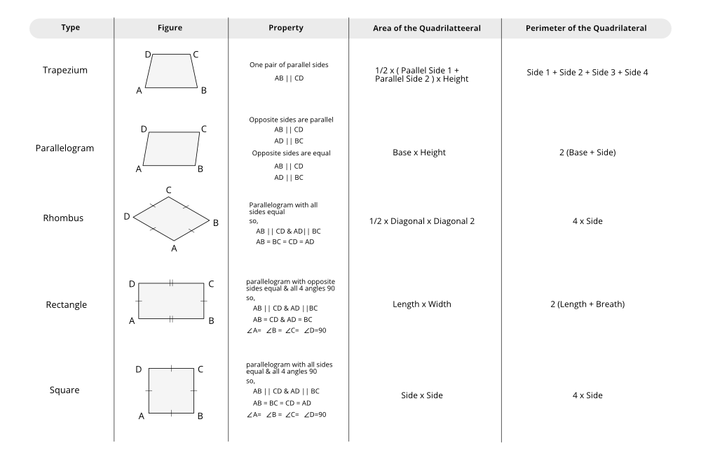
- Types of Quadrilateral: The measurements of the angles and lengths of the sides of quadrilaterals are used to classify them. The total space occupied by the figure is the quadrilateral’s area. The perimeter of a two-dimensional form is the entire distance covered by its boundaries. The following are the properties, area, and perimeter equations for the various quadrilaterals:
Chapter 4: Practical Geometry
This chapter is all about constructing quadrilateral. A quadrilateral is a geometrical figure that is a four-sided, four-angled polygon with two diagonals. For example square, rectangle, rhombus, etc.
To construct a quadrilateral uniquely, five measurements are required.
- A quadrilateral can be constructed uniquely if the lengths of its four sides and a diagonal are given.
- A quadrilateral can be constructed uniquely if its two diagonals and three sides are known.
- A quadrilateral can be constructed uniquely if its two adjacent sides and three angles are known.
- A quadrilateral can be constructed uniquely if its three sides and two included angles are given.
Chapter 5: Data Handling
Data handling refers to the process of collecting, organizing, and presenting any raw information in a way that is helpful to others like in graphs or charts, etc. Any problem that we need to study needs the collection of data, which must then be shown in such a manner that it provides a clear visual representation of the problem’s specifics while also examining the alternative solutions. Following are the list of the formulae and the important terms discussed in this chapter:
- Data: Data is a systematic record of facts or distinct values of a quantity.
- Arranging data in an order to study their salient features is called the presentation of data.
-
Frequency: It is defined as the number of times a particular entity occurs. A table is used to represent the frequency of different entities in the given data is termed a Frequency distribution table.
-
If the data present in the frequency distribution table is in the form of groups of the given values then it is called Grouped Frequency distribution table. This group data of the given values are grouped and called Class intervals. However, the number of values that each class contains is called the class size or width.
- The lower value in the class interval is called the Lower class limit.
- The upper value in the class interval is called the Upper-class limit.
-
Graphical representation of data:
- Pictograph: Pictorial representation of data using symbols.
- Bar Graph: A display of information using bars of uniform width, their heights proportional to the respective values.
- Double Bar Graph: A bar graph showing two sets of data simultaneously. It is useful for the comparison of the data.
- Histogram: a graphical representation of frequency distribution in the form of rectangles with class intervals as bases and heights proportional to corresponding frequencies such that there is no gap between any successive rectangles.
- Circle Graph or Pie Chart: A pictorial representation of the numerical data in the form of sectors of a circle such that area of each sector is proportional to the magnitude of the data represented by the sector.
- Probability = Number of outcomes making up an event / Total number of outcomes, if the outcomes are equally likely.
Chapter 6: Squares and Square Roots
A square number is a natural number (Let q) which can be expressed as p2, where n is also a natural number. e.g. 4 is square number as 4 = 22. The square root is the inverse operation of squaring.
If q is a natural number such that p2= q then,
√q = p and –p
Some of the important properties of Squares and Square roots are listed below:
- There are 2n non-perfect square numbers between n2 and (n+1)2.
- If a perfect square is of n digits then its square root will have n/2 digits if n is even, or (n+1)/2, if n is odd.
Chapter 7: Cubes and Cube roots
The inverse of the cube formula is the cube root formula. We multiply a number three times to obtain its cube in the cube formula, therefore in this situation, we break down a number to be written as a product of three equal numbers and get the cube root.
Consider any number m, which can be expressed as the product of any number three times as m = n × n × n = n3. n3 is so known as the cube of n and m is now known as cube root of n:
3√m = n
Method of finding a Cube Root: There are two different ways to determine the cube root of a number, that are:
- Prime Factorization Method
- Estimation Method
Chapter 8: Comparing Quantities
Class 8 Comparing Quantities formulas provided here have been thoroughly prepared by experts to assist students to understand all of the concepts and formulas used in Chapter 8. The below-mentioned formulas on some important topics like various Taxes such as sales Tax, Value Added Tax, Goods and Services Tax, Profit and Loss, Percent Change & Discounts are intended to assist students in completing timely modifications and achieving higher exam scores.
The following formulas will help students understand the basics of simple arithmetic involving money as,
- Profit = Selling price – Cost price
- Loss = Cost price – Selling price
- If SP > CP , then it is profit.
- If SP = CP , then it is neither profit nor loss.
- If CP > SP , then it is loss.
- Discount = Marked Price – Sale Price
- Discount % = Discount × 100 / MP
- Profit Percentage = (Profit / Cost Price) × 100
- Loss Percentage = (Loss / Cost Price) × 100
- Percentage Increased = Change in Value / Original Value
- Simple Interest = (Principal × Rate × Time)/100
- Compound Interest Formula = Amount – Principal
- Sales tax or VAT = Tax of Selling price = (Cost Price × Rate of Sales Tax) / 100
- Billing Amount = Selling price + VAT
Chapter 9: Algebraic Expressions and Identities
Algebraic expressions and algebraic identities are presented for class 8, this is a tough chapter in which you must memorize all of the equations and apply them correctly. GeeksforGeeks make it simple for them by putting all of the formulas on one page. Algebraic formulae and algebraic identities for class 8 are, we think, provided here.
These formulae will help students in learning fast and provide easy access to information when needed.
- (a + b)2 = a2 + 2ab + b2
- (a – b)2 = a2 – 2ab + b2
- (a + b) (a – b) = a2 – b2
- (x + a) (x + b) = x2 + (a + b)x + ab
- (x + a) (x – b) = x2 + (a – b)x – ab
- (x – a) (x + b) = x2 + (b – a)x – ab
- (x – a) (x – b) = x2 – (a + b)x + ab
- (a + b)3 = a3 + b3 + 3ab(a + b)
- (a – b)3 = a3 – b3 – 3ab(a – b)
Chapter 10: Visualising Solid Shapes
Solid geometry is vital in everyday life because it helps us comprehend the many forms we encounter and their properties. A comprehensive understanding of solid object visualization can help students master more sophisticated geometry principles and solve real-world situations. As a result, it’s critical to understand the numerous formulae related to various solids, which will aid in everyday computations.
Let’s learn about some important concepts and formulas used in this chapter
- Solids are defined by their form and the fact that they take up space. The faces of a solid are polygonal sections that make up the solid.
- Polyhedron: A polyhedron is a solid object bordered by polygons (platonic solid).
- Euler’s formula: A polyhedron has a certain number of planar faces, edges, and vertices that meet the formula:
F + V – E = 2
where F is the number of faces. The letters V and E stand for the number of vertices and edges, respectively.
- Prism: A prism is solid with parallelogram side faces and congruent parallel polygon ends (or bases). Two triangular faces, three rectangular faces, six vertices, and nine edges make up a prism.
- Pyramid: A pyramid is a polyhedron with a base that is a polygon with any number of sides and additional faces that are triangles with the same vertex. One square face, four triangular faces, five vertices, and eight edges make up a pyramid.
- Tetrahedron: If the base of a pyramid is a triangle, it is termed a triangular pyramid. The tetrahedron is another name for a triangular pyramid.
- Dimensions of a Solid: A solid item has three dimensions (measurements) – length, width, and height. Plane forms have two dimensions (measurements): length and breadth (or depth). As a result, they are referred to as two-dimensional and three-dimensional forms, respectively. They are referred to as two-dimensional and three-dimensional figures, respectively. Triangles, rectangles, and circles are two-dimensional forms, whereas cubes, cylinders, cones, and spheres are three-dimensional figures. From various angles, three-dimensional things appear to be different. As a result, they may be drawn from many angles, such as the top view, front view, and side view.
- Mapping: A map is not the same as a photograph. A map shows where one thing or place is in relation to other objects or locations. Symbols are used to represent various items and locations. On a map, there is no reference or perspective. Perspective, on the other hand, is critical when creating an image. Furthermore, maps have a scale that is set for each map.
- Faces, Vertices, and Edges: Faces are polygonal sections that make up a polyhedron. Edges are the line segments that connect the faces of a polyhedron. The vertices of a polyhedron are the spots where the edges cross. Three or more edges meet at a vertex of a polyhedron.
Chapter 11: Mensuration
The formulae for Mensuration Class 8 Chapter 11 are listed here. Here you will find mensuration resources based on the CBSE syllabus (2021-2022) and the most recent exam pattern. Work through the formulae and examples to have a better understanding of the idea of mensuration. Mensuration is the process of calculating the area and perimeter of various geometrical forms such as triangles, trapeziums, rectangles, and so on.
Chapter 12: Exponents and Powers
An exponent represents the value which refers to the number of times a number is multiplied by itself. For example, 5 × 5 × 5 can be written as 53. Even very small numbers can be expressed in the form of negative exponents. Here is a list of some of the laws related to exponents:
- Law of Product: am × an = am + n
- Law of Quotient: am/an = am – n
- Law of Zero Exponent: a0 = 1
- Law of Negative Exponent: a-m = 1/am
- Law of Power of a Power: (am)n = amn
- Law of Power of a Product: (ab)n = ambm
- Law of Power of a Quotient: (a/b)m = am/bm
Chapter 13: Direct and Inverse Proportions
To indicate how the quantities and amounts are connected to one another, a direct and inverse proportion is used. Direct proportional and inverse proportional are other terms used to describe them.
- Proportions: The proportionality is represented by the symbol ∝. For example, if we claim that p is proportional to q, this implies p ∝ q and if we say that p is inversely proportional to q, then this implies “p∝1/q.” Some proportionality rules govern these relations. Now, the value of ‘p’ changes in terms of ‘q’ in both circumstances, or when the value of ‘q’ changes, the value of ‘p’ changes as well. A proportionality constant is equal to the change in both values. Essentially, a proportion indicates that two ratios, such as p/q and r/s, are equivalent, i.e., p/q = r/s.
- Direct Proportion or Variation: Any two quantities a and b can be said to be in direct proportion if they variate (increase or decrease) together with each other in such a way that the ratio of their corresponding values remains the same. This implies that, If a/b = k, where k is any positive number, then a and b are said to be in direct proportion. e.g. If the number of things bought increases, then the total cost of purchase also increases.
- Quantities that increase or decrease in parallel do not necessarily have to be in direct proportion, and inverse proportion does not always have to be in direct proportion.
- Inverse Proportion: Two quantities x and y are said to be in inverse proportion if an increase in x causes a proportional decrease in y (and vice-versa) in such a manner that the product of their corresponding values remains constant. That is, if xy = k, then x and y are said to vary inversely. e.g. If the number of people increases, the time taken to finish the food decreases. Or If the speed will increase the time required to cover a given distance will decrease.
Chapter 14: Factorisation
Factorization is one of the most common ways for reducing an Algebraic or Quadratic Equation to its simplest form. As a result, one needs to be familiar with Factorization Formulas in order to decompose a complex equation. Below mentioned is the list of various formulas and properties that are useful to solve the problems of Polynomials, Trigonometry, Algebra, and Quadratic Equations.
- Factorisation: Factorization is the process of expressing an algebraic equation as a product of its components. Numbers, variables, or algebraic expressions can all be used as factors.
- Irreducible factor: A component that cannot be stated further as a product of factors is called irreducible.
-
Method to do Factorisation: The common factor approach is a method for factoring an equation in a methodical way. There are three steps to solve it:
- Each term of the statement should be written as a product of irreducible elements.
- Look for and separate the components that are similar.
- In each term, combine the remaining elements in line with the distributive law.
- All of the terms in a given expression may not share a common factor at times, but the terms can be grouped so that all of the terms in each group do. When we do this, a common factor emerges across all of the groups, resulting in the necessary factorization of the expression. This is the regrouping approach.
- When factoring by regrouping, keep in mind that any regrouping (i.e. rearrangement) of the terms in the provided equation may or may not result in factorization. We must observe the language and use trial and error to arrive at the desired regrouping.
-
A number of factorable expressions are of the form or may be factored into the form: a2 + 2ab + b2, a2 – 2ab + b2, a2 – b2 and x2 + (a + b)x + ab. These expressions can be easily factorized using below mentioned identities as,
- a2 + 2ab + b2 = (a + b)2
- a2 – 2ab + b2 = (a – b)2
- a2 – b2 = (a + b) (a – b)
- x2 + (a + b)x + ab = (x + a)(x + b)
- Remember that the numerical term yields ab in formulations with factors of the kind (x + a) (x + b). Its factors, a and b, should be chosen in such a way that their sum, with signs taken into account, equals the x coefficient.
- When dividing a polynomial by a monomial, we can divide the polynomial either by dividing each term by the monomial or by using the common factor technique.
- We can’t divide each term in the dividend polynomial by the divisor polynomial when dividing a polynomial by another polynomial. Instead, both polynomials are factored and their common factors are cancelled.
- We have divisions of algebraic expressions in the case of divisions of algebraic expressions that we discussed in this chapter.
Dividend = Divisor × Quotient
or
Dividend = Divisor × Quotient + Remainder
Chapter 15: Introduction to Graphs
The use of graphical tools to show data is particularly effective in organizing and comprehending the information. The following are some examples of graphical methods:
- When comparing categories, the bar graph is the most appropriate tool.
- Pie charts are the best way to compare sections of a whole.
- A histogram may be used to make data simpler to interpret when it is presented in intervals.
- A line graph will be beneficial in the situation of data that changes constantly over time.
- The x-coordinate and y-coordinate are required to fix a point on the graph sheet.
- A graph depicts the relationship between a dependent variable and an independent variable.
Chapter 16: Playing with Numbers
A number is said to be in general form if it can be stated as the sum of the products of its digits and their associated place values. Numbers can be written in a variety of ways. As a result, ab = 10a +b will be expressed as a two-digit number. In solving puzzles or playing number games, the general form of numbers is useful. When numbers are stated in general form, the reasons for divisibility by 10, 5, 2, 9, or 3 can be provided.
Rules for Divisibility:
- Divisibility by 2: A number is divisible by 2 when its one’s digit is 0, 2, 4, 6 or 8. e.g. 100a +10b +c here 100a and 10b are divisible by 2 because 100 and 10 are divisible by 2. Thus given number is divisible by 2 only when a = 0, 2, 4, 6 or 8.
- Divisibility by 3: A number is divisible by 3 when the sum of its digits is divisible by 3. e.g. 61785 the sum of digits = 6+1+7+8+5 = 27 which is divisible by 3. Therefore, 61785 is divisible 3.
- Divisibility by 4: A number is divisible by 4 when the number formed by its last two digits is divisible by 4. e.g.: 6216, 548, etc.
- Divisibility by 5: A number is divisible by 5 when its ones digit is 0 or 5. e.g.: 645, 540 etc.
- Divisibility by 6: A number is divisible by 6 when it is divisible by both 2 and 3. e.g.: 156, 5230, etc.
- Divisibility by 9: A number is divisible by 9 when the sum of its digits is divisible by 9. e.g.: consider a number 215847. Sum of digits = 2+1+5+8+4+7 = 27 which is divisible by 9. Therefore, 215847 is divisible by 9.
- Divisibility by 10: A number is divisible by 10 when its one digit is 0. e.g.: 540, 890, etc.
- Divisibility by 11: A number is divisible by 11 when the difference of the sum of its digits in odd places and the sum of its digits in even places is either o or a multiple of 11.
Share your thoughts in the comments
Please Login to comment...