This article discusses the basics of linear regression and its implementation in the Python programming language. Linear regression is a statistical method for modeling relationships between a dependent variable with a given set of independent variables.
Note: In this article, we refer to dependent variables as responses and independent variables as features for simplicity. In order to provide a basic understanding of linear regression, we start with the most basic version of linear regression, i.e. Simple linear regression.
What is Linear Regression?
Linear regression is a statistical method that is used to predict a continuous dependent variable(target variable) based on one or more independent variables(predictor variables). This technique assumes a linear relationship between the dependent and independent variables, which implies that the dependent variable changes proportionally with changes in the independent variables. In other words, linear regression is used to determine the extent to which one or more variables can predict the value of the dependent variable.
Assumptions We Make in a Linear Regression Model:
Given below are the basic assumptions that a linear regression model makes regarding a dataset on which it is applied:
- Linear relationship: The relationship between response and feature variables should be linear. The linearity assumption can be tested using scatter plots. As shown below, 1st figure represents linearly related variables whereas variables in the 2nd and 3rd figures are most likely non-linear. So, 1st figure will give better predictions using linear regression.

Linear relationship i the feature space
- Little or no multi-collinearity: It is assumed that there is little or no multicollinearity in the data. Multicollinearity occurs when the features (or independent variables) are not independent of each other.
- Little or no autocorrelation: Another assumption is that there is little or no autocorrelation in the data. Autocorrelation occurs when the residual errors are not independent of each other. You can refer here for more insight into this topic.
- No outliers: We assume that there are no outliers in the data. Outliers are data points that are far away from the rest of the data. Outliers can affect the results of the analysis.
- Homoscedasticity: Homoscedasticity describes a situation in which the error term (that is, the “noise” or random disturbance in the relationship between the independent variables and the dependent variable) is the same across all values of the independent variables. As shown below, figure 1 has homoscedasticity while Figure 2 has heteroscedasticity.

Homoscedasticity in Linear Regression
As we reach the end of this article, we discuss some applications of linear regression below.
Types of Linear Regression
There are two main types of linear regression:
- Simple linear regression: This involves predicting a dependent variable based on a single independent variable.
- Multiple linear regression: This involves predicting a dependent variable based on multiple independent variables.
Simple Linear Regression
Simple linear regression is an approach for predicting a response using a single feature. It is one of the most basic machine learning models that a machine learning enthusiast gets to know about. In linear regression, we assume that the two variables i.e. dependent and independent variables are linearly related. Hence, we try to find a linear function that predicts the response value(y) as accurately as possible as a function of the feature or independent variable(x). Let us consider a dataset where we have a value of response y for every feature x:
For generality, we define:
x as feature vector, i.e x = [x_1, x_2, …., x_n],
y as response vector, i.e y = [y_1, y_2, …., y_n]
for n observations (in the above example, n=10). A scatter plot of the above dataset looks like this:-
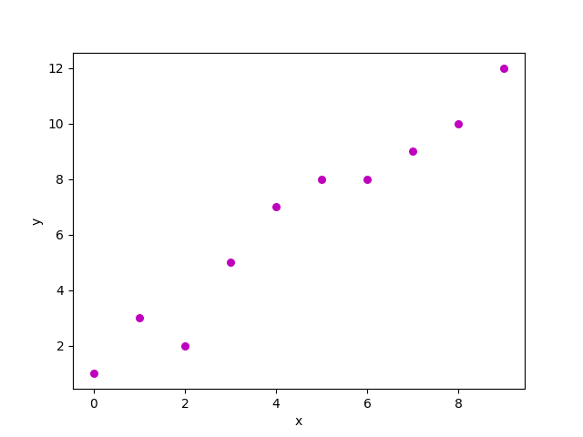
Scatter plot for the randomly generated data
Now, the task is to find a line that fits best in the above scatter plot so that we can predict the response for any new feature values. (i.e a value of x not present in a dataset) This line is called a regression line. The equation of the regression line is represented as:
[Tex]h(x_i) = \beta _0 + \beta_1x_i
[/Tex]
Here,
- h(x_i) represents the predicted response value for ith observation.
- b_0 and b_1 are regression coefficients and represent the y-intercept and slope of the regression line respectively.
To create our model, we must “learn” or estimate the values of regression coefficients b_0 and b_1. And once we’ve estimated these coefficients, we can use the model to predict responses!
In this article, we are going to use the principle of Least Squares.
Now consider:
[Tex]y_i = \beta_0 + \beta_1x_i + \varepsilon_i = h(x_i) + \varepsilon_i \Rightarrow \varepsilon_i = y_i -h(x_i)
[/Tex]
Here, e_i is a residual error in ith observation. So, our aim is to minimize the total residual error. We define the squared error or cost function, J as:
[Tex]J(\beta_0,\beta_1)= \frac{1}{2n} \sum_{i=1}^{n} \varepsilon_i^{2}
[/Tex]
And our task is to find the value of b0 and b1 for which J(b0, b1) is minimum! Without going into the mathematical details, we present the result here:
[Tex]\beta_1 = \frac{SS_{xy}}{SS_{xx}}
[/Tex]
[Tex]\beta_0 = \bar{y} – \beta_1\bar{x}
[/Tex]
Where SSxy is the sum of cross-deviations of y and x:
[Tex]SS_{xy} = \sum_{i=1}^{n} (x_i-\bar{x})(y_i-\bar{y}) = \sum_{i=1}^{n} y_ix_i – n\bar{x}\bar{y}
[/Tex]
And SSxx is the sum of squared deviations of x:
[Tex]SS_{xx} = \sum_{i=1}^{n} (x_i-\bar{x})^2 = \sum_{i=1}^{n}x_i^2 – n(\bar{x})^2
[/Tex]
Python Implementation of Simple Linear Regression
We can use the Python language to learn the coefficient of linear regression models. For plotting the input data and best-fitted line we will use the matplotlib library. It is one of the most used Python libraries for plotting graphs. Here is the example of simpe Linear regression using Python.
Importing Libraries
Python3
import numpy as np
import matplotlib.pyplot as plt
|
Estimating Coefficients Function
This function, estimate_coef(), takes the input data x (independent variable) and y (dependent variable) and estimates the coefficients of the linear regression line using the least squares method.
- Calculating Number of Observations:
n = np.size(x) determines the number of data points. - Calculating Means:
m_x = np.mean(x) and m_y = np.mean(y) compute the mean values of x and y, respectively. - Calculating Cross-Deviation and Deviation about x:
SS_xy = np.sum(y*x) - n*m_y*m_x and SS_xx = np.sum(x*x) - n*m_x*m_x calculate the sum of squared deviations between x and y and the sum of squared deviations of x about its mean, respectively. - Calculating Regression Coefficients:
b_1 = SS_xy / SS_xx and b_0 = m_y - b_1*m_x determine the slope (b_1) and intercept (b_0) of the regression line using the least squares method. - Returning Coefficients: The function returns the estimated coefficients as a tuple
(b_0, b_1).
Python3
def estimate_coef(x, y):
n = np.size(x)
m_x = np.mean(x)
m_y = np.mean(y)
SS_xy = np.sum(y*x) - n*m_y*m_x
SS_xx = np.sum(x*x) - n*m_x*m_x
b_1 = SS_xy / SS_xx
b_0 = m_y - b_1*m_x
return (b_0, b_1)
|
Plotting Regression Line Function
This function, plot_regression_line(), takes the input data x (independent variable), y (dependent variable), and the estimated coefficients b to plot the regression line and the data points.
- Plotting Scatter Plot:
plt.scatter(x, y, color = "m", marker = "o", s = 30) plots the original data points as a scatter plot with red markers. - Calculating Predicted Response Vector:
y_pred = b[0] + b[1]*x calculates the predicted values for y based on the estimated coefficients b. - Plotting Regression Line:
plt.plot(x, y_pred, color = "g") plots the regression line using the predicted values and the independent variable x. - Adding Labels:
plt.xlabel('x') and plt.ylabel('y') label the x-axis as 'x' and the y-axis as 'y', respectively.
Python3
def plot_regression_line(x, y, b):
plt.scatter(x, y, color = "m",
marker = "o", s = 30)
y_pred = b[0] + b[1]*x
plt.plot(x, y_pred, color = "g")
plt.xlabel('x')
plt.ylabel('y')
|
Output:
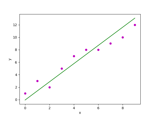
Scatterplot of the points along with the regression line
Main Function
The provided code implements simple linear regression analysis by defining a function main() that performs the following steps:
- Data Definition: Defines the independent variable (
x) and dependent variable (y) as NumPy arrays. - Coefficient Estimation: Calls the
estimate_coef() function to determine the coefficients of the linear regression line using the provided data. - Printing Coefficients: Prints the estimated intercept (
b_0) and slope (b_1) of the regression line.
Python3
def main():
x = np.array([0, 1, 2, 3, 4, 5, 6, 7, 8, 9])
y = np.array([1, 3, 2, 5, 7, 8, 8, 9, 10, 12])
b = estimate_coef(x, y)
print("Estimated coefficients:\nb_0 = {} \
\nb_1 = {}".format(b
|
Output:
Estimated coefficients:
b_0 = -0.0586206896552
b_1 = 1.45747126437
Multiple Linear Regression
Multiple linear regression attempts to model the relationship between two or more features and a response by fitting a linear equation to the observed data.
Clearly, it is nothing but an extension of simple linear regression. Consider a dataset with p features(or independent variables) and one response(or dependent variable).
Also, the dataset contains n rows/observations.
We define:
X (feature matrix) = a matrix of size n X p where xij denotes the values of the jth feature for ith observation.
So,
[Tex]\begin{pmatrix} x_{11} & \cdots & x_{1p} \\ x_{21} & \cdots & x_{2p} \\ \vdots & \ddots & \vdots \\ x_{n1} & \vdots & x_{np} \end{pmatrix}
[/Tex]
and
y (response vector) = a vector of size n where y_{i} denotes the value of response for ith observation.
[Tex]y = \begin{bmatrix} y_1\\ y_2\\ .\\ .\\ y_n \end{bmatrix}
[/Tex]
The regression line for p features is represented as:
[Tex]h(x_i) = \beta_0 + \beta_1x_{i1} + \beta_2x_{i2} + …. + \beta_px_{ip}
[/Tex]
where h(x_i) is predicted response value for ith observation and b_0, b_1, …, b_p are the regression coefficients. Also, we can write:
[Tex]\newline y_i = \beta_0 + \beta_1x_{i1} + \beta_2x_{i2} + …. + \beta_px_{ip} + \varepsilon_i \newline or \newline y_i = h(x_i) + \varepsilon_i \Rightarrow \varepsilon_i = y_i – h(x_i)
[/Tex]
where e_i represents a residual error in ith observation. We can generalize our linear model a little bit more by representing feature matrix X as:
[Tex]X = \begin{pmatrix} 1 & x_{11} & \cdots & x_{1p} \\ 1 & x_{21} & \cdots & x_{2p} \\ \vdots & \vdots & \ddots & \vdots \\ 1 & x_{n1} & \cdots & x_{np} \end{pmatrix}
[/Tex]
So now, the linear model can be expressed in terms of matrices as:
[Tex]y = X\beta + \varepsilon
[/Tex]
where,
[Tex]\beta = \begin{bmatrix} \beta_0\\ \beta_1\\ .\\ .\\ \beta_p \end{bmatrix}
[/Tex]
and
[Tex]\varepsilon = \begin{bmatrix} \varepsilon_1\\ \varepsilon_2\\ .\\ .\\ \varepsilon_n \end{bmatrix}
[/Tex]
Now, we determine an estimate of b, i.e. b’ using the Least Squares method. As already explained, the Least Squares method tends to determine b’ for which total residual error is minimized.
We present the result directly here:
[Tex]\hat{\beta} = ({X}’X)^{-1} {X}’y
[/Tex]
where ‘ represents the transpose of the matrix while -1 represents the matrix inverse. Knowing the least square estimates, b’, the multiple linear regression model can now be estimated as:
[Tex]\hat{y} = X\hat{\beta}
[/Tex]
where y’ is the estimated response vector.
Python Implementation of Multiple Linear Regression
For multiple linear regression using Python, we will use the Boston house pricing dataset.
Importing Libraries
Python3
from sklearn.model_selection import train_test_split
import matplotlib.pyplot as plt
import numpy as np
from sklearn import datasets, linear_model, metrics
import pandas as pd
|
Loading the Boston Housing Dataset
The code downloads the Boston Housing dataset from the provided URL and reads it into a Pandas DataFrame (raw_df)
Python3
raw_df = pd.read_csv(data_url, sep="\s+",
skiprows=22, header=None)
|
Preprocessing Data
This extracts the input variables (X) and target variable (y) from the DataFrame. The input variables are selected from every other row to match the target variable, which is available every other row.
Python3
X = np.hstack([raw_df.values[::2, :],
raw_df.values[1::2, :2]])
y = raw_df.values[1::2, 2]
|
Splitting Data into Training and Testing Sets
Here it divides the data into training and testing sets using the train_test_split() function from scikit-learn. The test_size parameter specifies that 40% of the data should be used for testing.
Python3
X_train, X_test,\
y_train, y_test = train_test_split(X, y,
test_size=0.4,
random_state=1)
|
Creating and Training the Linear Regression Model
This initializes a LinearRegression object (reg) and trains the model using the training data (X_train, y_train)
Python3
reg = linear_model.LinearRegression()
reg.fit(X_train, y_train)
|
Evaluating Model Performance
Evaluates the model’s performance by printing the regression coefficients and calculating the variance score, which measures the proportion of explained variance. A score of 1 indicates perfect prediction.
Python3
print('Coefficients: ', reg.coef_)
print('Variance score: {}'.format(reg.score(X_test, y_test)))
|
Output:
Coefficients:
[ -8.80740828e-02 6.72507352e-02 5.10280463e-02 2.18879172e+00
-1.72283734e+01 3.62985243e+00 2.13933641e-03 -1.36531300e+00
2.88788067e-01 -1.22618657e-02 -8.36014969e-01 9.53058061e-03
-5.05036163e-01]
Variance score: 0.720898784611
Plotting Residual Errors
Plotting and analyzing the residual errors, which represent the difference between the predicted values and the actual values.
Python3
plt.style.use('fivethirtyeight')
plt.scatter(reg.predict(X_train),
reg.predict(X_train) - y_train,
color="green", s=10,
label='Train data')
plt.scatter(reg.predict(X_test),
reg.predict(X_test) - y_test,
color="blue", s=10,
label='Test data')
plt.hlines(y=0, xmin=0, xmax=50, linewidth=2)
plt.legend(loc='upper right')
plt.title("Residual errors")
plt.show()
|
Output:
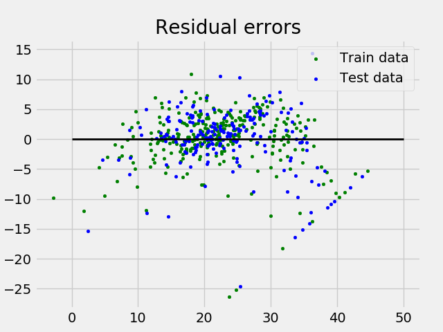
Residual Error Plot for the Multiple Linear Regression
In the above example, we determine the accuracy score using Explained Variance Score. We define:
explained_variance_score = 1 – Var{y – y’}/Var{y}
where y’ is the estimated target output, y is the corresponding (correct) target output, and Var is Variance, the square of the standard deviation. The best possible score is 1.0, lower values are worse.
Polynomial Linear Regression
Polynomial Regression is a form of linear regression in which the relationship between the independent variable x and dependent variable y is modeled as an nth-degree polynomial. Polynomial regression fits a nonlinear relationship between the value of x and the corresponding conditional mean of y, denoted E(y | x).
Choosing a Degree for Polynomial Regression
The choice of degree for polynomial regression is a trade-off between bias and variance. Bias is the tendency of a model to consistently predict the same value, regardless of the true value of the dependent variable. Variance is the tendency of a model to make different predictions for the same data point, depending on the specific training data used.
A higher-degree polynomial can reduce bias but can also increase variance, leading to overfitting. Conversely, a lower-degree polynomial can reduce variance but can also increase bias.
There are a number of methods for choosing a degree for polynomial regression, such as cross-validation and using information criteria such as Akaike information criterion (AIC) or Bayesian information criterion (BIC).
Implementation of Polynomial Regression using Python
Implementing the Polynomial regression using Python:
Here we will import all the necessary libraries for data analysis and machine learning tasks and then loads the ‘Position_Salaries.csv’ dataset using Pandas. It then prepares the data for modeling by handling missing values and encoding categorical data. Finally, it splits the data into training and testing sets and standardizes the numerical features using StandardScaler.
Python3
import pandas as pd
import matplotlib.pyplot as plt
import seaborn as sns
import sklearn
import warnings
from sklearn.preprocessing import LabelEncoder
from sklearn.impute import KNNImputer
from sklearn.model_selection import train_test_split
from sklearn.preprocessing import StandardScaler
from sklearn.metrics import f1_score
from sklearn.ensemble import RandomForestRegressor
from sklearn.ensemble import RandomForestRegressor
from sklearn.model_selection import cross_val_score
warnings.filterwarnings('ignore')
df = pd.read_csv('Position_Salaries.csv')
X = df.iloc[:,1:2].values
y = df.iloc[:,2].values
x
|
Output:
array([[ 1, 45000, 0],
[ 2, 50000, 4],
[ 3, 60000, 8],
[ 4, 80000, 5],
[ 5, 110000, 3],
[ 6, 150000, 7],
[ 7, 200000, 6],
[ 8, 300000, 9],
[ 9, 500000, 1],
[ 10, 1000000, 2]], dtype=int64)
The code creates a linear regression model and fits it to the provided data, establishing a linear relationship between the independent and dependent variables.
Python3
from sklearn.linear_model import LinearRegression
lin_reg=LinearRegression()
lin_reg.fit(X,y)
|
The code performs quadratic and cubic regression by generating polynomial features from the original data and fitting linear regression models to these features. This enables modeling nonlinear relationships between the independent and dependent variables.
Python3
from sklearn.preprocessing import PolynomialFeatures
poly_reg2=PolynomialFeatures(degree=2)
X_poly=poly_reg2.fit_transform(X)
lin_reg_2=LinearRegression()
lin_reg_2.fit(X_poly,y)
poly_reg3=PolynomialFeatures(degree=3)
X_poly3=poly_reg3.fit_transform(X)
lin_reg_3=LinearRegression()
lin_reg_3.fit(X_poly3,y)
|
The code creates a scatter plot of the data point, It effectively visualizes the linear relationship between position level and salary.
Python3
plt.scatter(X,y,color='red')
plt.plot(X,lin_reg.predict(X),color='green')
plt.title('Simple Linear Regression')
plt.xlabel('Position Level')
plt.ylabel('Salary')
plt.show()
|
Output:

The code creates a scatter plot of the data points, overlays the predicted quadratic and cubic regression lines. It effectively visualizes the nonlinear relationship between position level and salary and compares the fits of quadratic and cubic regression models.
Python3
plt.style.use('fivethirtyeight')
plt.scatter(X,y,color='red')
plt.plot(X,lin_reg_2.predict(poly_reg2.fit_transform(X)),color='green')
plt.plot(X,lin_reg_3.predict(poly_reg3.fit_transform(X)),color='yellow')
plt.title('Polynomial Linear Regression Degree 2')
plt.xlabel('Position Level')
plt.ylabel('Salary')
plt.show()
|
Output:

The code effectively visualizes the relationship between position level and salary using cubic regression and generates a continuous prediction line for a broader range of position levels.
Python3
plt.style.use('fivethirtyeight')
X_grid=np.arange(min(X),max(X),0.1)
X_grid=X_grid.reshape((len(X_grid),1))
plt.scatter(X,y,color='red')
plt.plot(X_grid,lin_reg_3.predict(poly_reg3.fit_transform(X_grid)),color='lightgreen')
plt.title('Polynomial Linear Regression Degree 3')
plt.xlabel('Position Level')
plt.ylabel('Salary')
plt.show()
|
Output:

Applications of Linear Regression
- Trend lines: A trend line represents the variation in quantitative data with the passage of time (like GDP, oil prices, etc.). These trends usually follow a linear relationship. Hence, linear regression can be applied to predict future values. However, this method suffers from a lack of scientific validity in cases where other potential changes can affect the data.
- Economics: Linear regression is the predominant empirical tool in economics. For example, it is used to predict consumer spending, fixed investment spending, inventory investment, purchases of a country’s exports, spending on imports, the demand to hold liquid assets, labor demand, and labor supply.
- Finance: The capital price asset model uses linear regression to analyze and quantify the systematic risks of an investment.
- Biology: Linear regression is used to model causal relationships between parameters in biological systems.
Advantages of Linear Regression
- Easy to interpret: The coefficients of a linear regression model represent the change in the dependent variable for a one-unit change in the independent variable, making it simple to comprehend the relationship between the variables.
- Robust to outliers: Linear regression is relatively robust to outliers meaning it is less affected by extreme values of the independent variable compared to other statistical methods.
- Can handle both linear and nonlinear relationships: Linear regression can be used to model both linear and nonlinear relationships between variables. This is because the independent variable can be transformed before it is used in the model.
- No need for feature scaling or transformation: Unlike some machine learning algorithms, linear regression does not require feature scaling or transformation. This can be a significant advantage, especially when dealing with large datasets.
Disadvantages of Linear Regression
- Assumes linearity: Linear regression assumes that the relationship between the independent variable and the dependent variable is linear. This assumption may not be valid for all data sets. In cases where the relationship is nonlinear, linear regression may not be a good choice.
- Sensitive to multicollinearity: Linear regression is sensitive to multicollinearity. This occurs when there is a high correlation between the independent variables. Multicollinearity can make it difficult to interpret the coefficients of the model and can lead to overfitting.
- May not be suitable for highly complex relationships: Linear regression may not be suitable for modeling highly complex relationships between variables. For example, it may not be able to model relationships that include interactions between the independent variables.
- Not suitable for classification tasks: Linear regression is a regression algorithm and is not suitable for classification tasks, which involve predicting a categorical variable rather than a continuous variable.
Frequently Asked Question(FAQs)
1. How to use linear regression to make predictions?
Once a linear regression model has been trained, it can be used to make predictions for new data points. The scikit-learn LinearRegression class provides a method called predict() that can be used to make predictions.
2.What is linear regression?
Linear regression is a supervised machine learning algorithm used to predict a continuous numerical output. It assumes that the relationship between the independent variables (features) and the dependent variable (target) is linear, meaning that the predicted value of the target can be calculated as a linear combination of the features.
3. How to perform linear regression in Python?
There are several libraries in Python that can be used to perform linear regression, including scikit-learn, statsmodels, and NumPy. The scikit-learn library is the most popular choice for machine learning tasks, and it provides a simple and efficient implementation of linear regression.
4. What are some applications of linear regression?
Linear regression is a versatile algorithm that can be used for a wide variety of applications, including finance, healthcare, and marketing. Some specific examples include:
- Predicting house prices
- Predicting stock prices
- Diagnosing medical conditions
- Predicting customer churn
5. How linear regression is implemented in sklearn?
Linear regression is implemented in scikit-learn using the LinearRegression class. This class provides methods to fit a linear regression model to a training dataset and predict the target value for new data points.
Share your thoughts in the comments
Please Login to comment...