Python | Linear Regression using sklearn
Last Updated :
02 Aug, 2023
Prerequisite: Linear Regression
Linear Regression is a machine learning algorithm based on supervised learning. It performs a regression task. Regression models a target prediction value based on independent variables. It is mostly used for finding out the relationship between variables and forecasting. Different regression models differ based on – the kind of relationship between the dependent and independent variables, they are considering and the number of independent variables being used. This article is going to demonstrate how to use the various Python libraries to implement linear regression on a given dataset. We will demonstrate a binary linear model as this will be easier to visualize. In this demonstration, the model will use Gradient Descent to learn. You can learn about it here.
Step 1: Importing all the required libraries
Python3
import numpy as np
import pandas as pd
import seaborn as sns
import matplotlib.pyplot as plt
from sklearn import preprocessing, svm
from sklearn.model_selection import train_test_split
from sklearn.linear_model import LinearRegression
|
Step 2: Reading the dataset You can download the dataset
Python3
df = pd.read_csv('bottle.csv')
df_binary = df[['Salnty', 'T_degC']]
df_binary.columns = ['Sal', 'Temp']
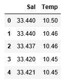
df_binary.head()
|
Output:
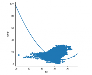
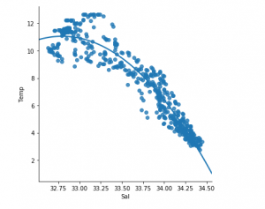
Step 3: Exploring the data scatter
Python3
sns.lmplot(x ="Sal", y ="Temp", data = df_binary, order = 2, ci = None)
plt.show()
|
Output:
Step 4: Data cleaning
Python3
df_binary.fillna(method ='ffill', inplace = True)
|
Step 5: Training our model
Python3
X = np.array(df_binary['Sal']).reshape(-1, 1)
y = np.array(df_binary['Temp']).reshape(-1, 1)
df_binary.dropna(inplace = True)
X_train, X_test, y_train, y_test = train_test_split(X, y, test_size = 0.25)
regr = LinearRegression()
regr.fit(X_train, y_train)
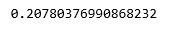
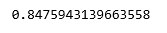
print(regr.score(X_test, y_test))
|
Output:
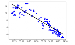
Step 6: Exploring our results
Python3
y_pred = regr.predict(X_test)
plt.scatter(X_test, y_test, color ='b')
plt.plot(X_test, y_pred, color ='k')
plt.show()
|
Output:
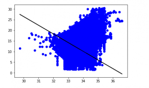
The low accuracy score of our model suggests that our regressive model has not fit very well with the existing data. This suggests that our data is not suitable for linear regression. But sometimes, a dataset may accept a linear regressor if we consider only a part of it. Let us check for that possibility.
Step 7: Working with a smaller dataset
Python3
df_binary500 = df_binary[:][:500]
sns.lmplot(x ="Sal", y ="Temp", data = df_binary500,
order = 2, ci = None)
|
Output:
We can already see that the first 500 rows follow a linear model. Continuing with the same steps as before.
Python3
df_binary500.fillna(method ='fill', inplace = True)
X = np.array(df_binary500['Sal']).reshape(-1, 1)
y = np.array(df_binary500['Temp']).reshape(-1, 1)
df_binary500.dropna(inplace = True)
X_train, X_test, y_train, y_test = train_test_split(X, y, test_size = 0.25)
regr = LinearRegression()
regr.fit(X_train, y_train)
print(regr.score(X_test, y_test))
|
Output:
Python3
y_pred = regr.predict(X_test)
plt.scatter(X_test, y_test, color ='b')
plt.plot(X_test, y_pred, color ='k')
plt.show()
|
Output:
Step 8: Evaluation Metrics For Regression
At last, we check the performance of the Linear Regression model with help of evaluation metrics. For Regression algorithms we widely use mean_absolute_error, and mean_squared_error metrics to check the model performance.
Python3
from sklearn.metrics import mean_absolute_error,mean_squared_error
mae = mean_absolute_error(y_true=y_test,y_pred=y_pred)
mse = mean_squared_error(y_true=y_test,y_pred=y_pred)
rmse = mean_squared_error(y_true=y_test,y_pred=y_pred,squared=False)
print("MAE:",mae)
print("MSE:",mse)
print("RMSE:",rmse)
|
Output:
MAE: 0.7927322046360309
MSE: 1.0251137190180517
RMSE: 1.0124789968281078
Share your thoughts in the comments
Please Login to comment...