Logistic Regression in Machine Learning

Logistic regression is a supervised machine learning algorithm used for classification tasks where the goal is to predict the probability that an instance belongs to a given class or not. Logistic regression is a statistical algorithm which analyze the relationship between two data factors. The article explores the fundamentals of logistic regression, it’s types and implementations.

What is Logistic Regression?

Logistic regression is used for binary classification where we use sigmoid function, that takes input as independent variables and produces a probability value between 0 and 1.

For example, we have two classes Class 0 and Class 1 if the value of the logistic function for an input is greater than 0.5 (threshold value) then it belongs to Class 1 otherwise it belongs to Class 0. It’s referred to as regression because it is the extension of linear regression but is mainly used for classification problems.

Key Points:

• Logistic regression predicts the output of a categorical dependent variable. Therefore, the outcome must be a categorical or discrete value.
• It can be either Yes or No, 0 or 1, true or False, etc. but instead of giving the exact value as 0 and 1, it gives the probabilistic values which lie between 0 and 1.
• In Logistic regression, instead of fitting a regression line, we fit an “S” shaped logistic function, which predicts two maximum values (0 or 1).

Logistic Function – Sigmoid Function

• The sigmoid function is a mathematical function used to map the predicted values to probabilities.
• It maps any real value into another value within a range of 0 and 1. The value of the logistic regression must be between 0 and 1, which cannot go beyond this limit, so it forms a curve like the “S” form.
• The S-form curve is called the Sigmoid function or the logistic function.
• In logistic regression, we use the concept of the threshold value, which defines the probability of either 0 or 1. Such as values above the threshold value tends to 1, and a value below the threshold values tends to 0.

Types of Logistic Regression

On the basis of the categories, Logistic Regression can be classified into three types:

1. Binomial: In binomial Logistic regression, there can be only two possible types of the dependent variables, such as 0 or 1, Pass or Fail, etc.
2. Multinomial: In multinomial Logistic regression, there can be 3 or more possible unordered types of the dependent variable, such as “cat”, “dogs”, or “sheep”
3. Ordinal: In ordinal Logistic regression, there can be 3 or more possible ordered types of dependent variables, such as “low”, “Medium”, or “High”.

Assumptions of Logistic Regression

We will explore the assumptions of logistic regression as understanding these assumptions is important to ensure that we are using appropriate application of the model. The assumption include:

1. Independent observations: Each observation is independent of the other. meaning there is no correlation between any input variables.
2. Binary dependent variables: It takes the assumption that the dependent variable must be binary or dichotomous, meaning it can take only two values. For more than two categories SoftMax functions are used.
3. Linearity relationship between independent variables and log odds: The relationship between the independent variables and the log odds of the dependent variable should be linear.
4. No outliers: There should be no outliers in the dataset.
5. Large sample size: The sample size is sufficiently large

Terminologies involved in Logistic Regression

Here are some common terms involved in logistic regression:

• Independent variables: The input characteristics or predictor factors applied to the dependent variable’s predictions.
• Dependent variable: The target variable in a logistic regression model, which we are trying to predict.
• Logistic function: The formula used to represent how the independent and dependent variables relate to one another. The logistic function transforms the input variables into a probability value between 0 and 1, which represents the likelihood of the dependent variable being 1 or 0.
• Odds: It is the ratio of something occurring to something not occurring. it is different from probability as the probability is the ratio of something occurring to everything that could possibly occur.
• Log-odds: The log-odds, also known as the logit function, is the natural logarithm of the odds. In logistic regression, the log odds of the dependent variable are modeled as a linear combination of the independent variables and the intercept.
• Coefficient: The logistic regression model’s estimated parameters, show how the independent and dependent variables relate to one another.
• Intercept: A constant term in the logistic regression model, which represents the log odds when all independent variables are equal to zero.
• Maximum likelihood estimation: The method used to estimate the coefficients of the logistic regression model, which maximizes the likelihood of observing the data given the model.

How does Logistic Regression work?

The logistic regression model transforms the linear regression function continuous value output into categorical value output using a sigmoid function, which maps any real-valued set of independent variables input into a value between 0 and 1. This function is known as the logistic function.

Let the independent input features be:

[Tex]X = \begin{bmatrix} x_{11}  & … & x_{1m}\\ x_{21}  & … & x_{2m} \\  \vdots & \ddots  & \vdots  \\ x_{n1}  & … & x_{nm} \end{bmatrix}[/Tex]

 and the dependent variable is Y having only binary value i.e. 0 or 1. 

[Tex]Y = \begin{cases} 0 & \text{ if } Class\;1 \\ 1 & \text{ if } Class\;2 \end{cases} [/Tex]

then, apply the multi-linear function to the input variables X.

[Tex]z = \left(\sum_{i=1}^{n} w_{i}x_{i}\right) + b [/Tex]

Here [Tex]x_i [/Tex] is the ith observation of X, [Tex]w_i = [w_1, w_2, w_3, \cdots,w_m] [/Tex] is the weights or Coefficient, and b is the bias term also known as intercept. simply this can be represented as the dot product of weight and bias.

[Tex]z = w\cdot X +b [/Tex]

whatever we discussed above is the linear regression. 

Sigmoid Function

Now we use the sigmoid function where the input will be z and we find the probability between 0 and 1. i.e. predicted y.

[Tex]\sigma(z) = \frac{1}{1-e^{-z}} [/Tex]

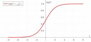
Sigmoid function

As shown above, the figure sigmoid function converts the continuous variable data into the probability i.e. between 0 and 1. 

• [Tex]\sigma(z)    [/Tex] tends towards 1 as [Tex]z\rightarrow\infty [/Tex]
• [Tex]\sigma(z)    [/Tex] tends towards 0 as [Tex]z\rightarrow-\infty [/Tex]
• [Tex]\sigma(z)    [/Tex] is always bounded between 0 and 1

where the probability of being a class can be measured as:

[Tex]P(y=1) = \sigma(z) \\ P(y=0) = 1-\sigma(z) [/Tex]

Logistic Regression Equation

The odd is the ratio of something occurring to something not occurring. it is different from probability as the probability is the ratio of something occurring to everything that could possibly occur. so odd will be:

[Tex]\frac{p(x)}{1-p(x)}  = e^z[/Tex]

Applying natural log on odd. then log odd will be:

[Tex]\begin{aligned} \log \left[\frac{p(x)}{1-p(x)} \right] &= z \\ \log \left[\frac{p(x)}{1-p(x)} \right] &= w\cdot X +b \\ \frac{p(x)}{1-p(x)}&= e^{w\cdot X +b} \;\;\cdots\text{Exponentiate both sides} \\ p(x) &=e^{w\cdot X +b}\cdot (1-p(x)) \\p(x) &=e^{w\cdot X +b}-e^{w\cdot X +b}\cdot p(x)) \\p(x)+e^{w\cdot X +b}\cdot p(x))&=e^{w\cdot X +b} \\p(x)(1+e^{w\cdot X +b}) &=e^{w\cdot X +b} \\p(x)&= \frac{e^{w\cdot X +b}}{1+e^{w\cdot X +b}} \end{aligned}[/Tex]

then the final logistic regression equation will be:

[Tex]p(X;b,w) = \frac{e^{w\cdot X +b}}{1+e^{w\cdot X +b}} = \frac{1}{1+e^{-w\cdot X +b}}[/Tex]

Likelihood Function for Logistic Regression

The predicted probabilities will be:

• for y=1 The predicted probabilities will be: p(X;b,w) = p(x)
• for y = 0 The predicted probabilities will be: 1-p(X;b,w) = 1-p(x)

[Tex]L(b,w) = \prod_{i=1}^{n}p(x_i)^{y_i}(1-p(x_i))^{1-y_i}[/Tex]

Taking natural logs on both sides

[Tex]\begin{aligned}\log(L(b,w)) &= \sum_{i=1}^{n} y_i\log p(x_i)\;+\; (1-y_i)\log(1-p(x_i)) \\ &=\sum_{i=1}^{n} y_i\log p(x_i)+\log(1-p(x_i))-y_i\log(1-p(x_i)) \\ &=\sum_{i=1}^{n} \log(1-p(x_i)) +\sum_{i=1}^{n}y_i\log \frac{p(x_i)}{1-p(x_i} \\ &=\sum_{i=1}^{n} -\log1-e^{-(w\cdot x_i+b)} +\sum_{i=1}^{n}y_i (w\cdot x_i +b) \\ &=\sum_{i=1}^{n} -\log1+e^{w\cdot x_i+b} +\sum_{i=1}^{n}y_i (w\cdot x_i +b) \end{aligned}[/Tex]

Gradient of the log-likelihood function

To find the maximum likelihood estimates, we differentiate w.r.t w,

[Tex]\begin{aligned} \frac{\partial J(l(b,w)}{\partial w_j}&=-\sum_{i=n}^{n}\frac{1}{1+e^{w\cdot x_i+b}}e^{w\cdot x_i+b} x_{ij} +\sum_{i=1}^{n}y_{i}x_{ij} \\&=-\sum_{i=n}^{n}p(x_i;b,w)x_{ij}+\sum_{i=1}^{n}y_{i}x_{ij} \\&=\sum_{i=n}^{n}(y_i -p(x_i;b,w))x_{ij} \end{aligned} [/Tex]

Code Implementation for Logistic Regression

Binomial Logistic regression:

Target variable can have only 2 possible types: “0” or “1” which may represent “win” vs “loss”, “pass” vs “fail”, “dead” vs “alive”, etc., in this case, sigmoid functions are used, which is already discussed above.

Importing necessary libraries based on the requirement of model. This Python code shows how to use the breast cancer dataset to implement a Logistic Regression model for classification.

Python3

# import the necessary libraries from sklearn.datasets import load_breast_cancer from sklearn.linear_model import LogisticRegression from sklearn.model_selection import train_test_split from sklearn.metrics import accuracy_score # load the breast cancer dataset X, y = load_breast_cancer(return_X_y=True) # split the train and test dataset X_train, X_test,\ y_train, y_test = train_test_split(X, y, test_size=0.20, random_state=23) # LogisticRegression clf = LogisticRegression(random_state=0) clf.fit(X_train, y_train) # Prediction y_pred = clf.predict(X_test) acc = accuracy_score(y_test, y_pred) print("Logistic Regression model accuracy (in %):", acc*100)

Output:

Logistic Regression model accuracy (in %): 95.6140350877193

Multinomial Logistic Regression:

Target variable can have 3 or more possible types which are not ordered (i.e. types have no quantitative significance) like “disease A” vs “disease B” vs “disease C”.

In this case, the softmax function is used in place of the sigmoid function. Softmax function for K classes will be:

[Tex]\text{softmax}(z_i) =\frac{ e^{z_i}}{\sum_{j=1}^{K}e^{z_{j}}}[/Tex]

Here, K represents the number of elements in the vector z, and i, j iterates over all the elements in the vector.

Then the probability for class c will be:

[Tex]P(Y=c | \overrightarrow{X}=x) = \frac{e^{w_c \cdot x + b_c}}{\sum_{k=1}^{K}e^{w_k \cdot x + b_k}}[/Tex]

In Multinomial Logistic Regression, the output variable can have more than two possible discrete outputs. Consider the Digit Dataset. 

Python3

from sklearn.model_selection import train_test_split from sklearn import datasets, linear_model, metrics # load the digit dataset digits = datasets.load_digits() # defining feature matrix(X) and response vector(y) X = digits.data y = digits.target # splitting X and y into training and testing sets X_train, X_test,\ y_train, y_test = train_test_split(X, y, test_size=0.4, random_state=1) # create logistic regression object reg = linear_model.LogisticRegression() # train the model using the training sets reg.fit(X_train, y_train) # making predictions on the testing set y_pred = reg.predict(X_test) # comparing actual response values (y_test) # with predicted response values (y_pred) print("Logistic Regression model accuracy(in %):", metrics.accuracy_score(y_test, y_pred)*100)

Output:

Logistic Regression model accuracy(in %): 96.52294853963839

How to Evaluate Logistic Regression Model?

We can evaluate the logistic regression model using the following metrics:

• Accuracy: Accuracy provides the proportion of correctly classified instances.
  [Tex]Accuracy = \frac{True \, Positives + True \, Negatives}{Total} [/Tex]

• Precision: Precision focuses on the accuracy of positive predictions.
  [Tex]Precision = \frac{True \, Positives }{True\, Positives + False \, Positives} [/Tex]

• Recall (Sensitivity or True Positive Rate): Recall measures the proportion of correctly predicted positive instances among all actual positive instances.
  [Tex]Recall = \frac{ True \, Positives}{True\, Positives + False \, Negatives} [/Tex]

• F1 Score: F1 score is the harmonic mean of precision and recall.
  [Tex]F1 \, Score = 2 * \frac{Precision * Recall}{Precision + Recall} [/Tex]

• Area Under the Receiver Operating Characteristic Curve (AUC-ROC): The ROC curve plots the true positive rate against the false positive rate at various thresholds. AUC-ROC measures the area under this curve, providing an aggregate measure of a model’s performance across different classification thresholds.
• Area Under the Precision-Recall Curve (AUC-PR): Similar to AUC-ROC, AUC-PR measures the area under the precision-recall curve, providing a summary of a model’s performance across different precision-recall trade-offs.

Precision-Recall Tradeoff in Logistic Regression Threshold Setting

Logistic regression becomes a classification technique only when a decision threshold is brought into the picture. The setting of the threshold value is a very important aspect of Logistic regression and is dependent on the classification problem itself.

The decision for the value of the threshold value is majorly affected by the values of precision and recall. Ideally, we want both precision and recall being 1, but this seldom is the case.

In the case of a Precision-Recall tradeoff, we use the following arguments to decide upon the threshold:

1. Low Precision/High Recall: In applications where we want to reduce the number of false negatives without necessarily reducing the number of false positives, we choose a decision value that has a low value of Precision or a high value of Recall. For example, in a cancer diagnosis application, we do not want any affected patient to be classified as not affected without giving much heed to if the patient is being wrongfully diagnosed with cancer. This is because the absence of cancer can be detected by further medical diseases, but the presence of the disease cannot be detected in an already rejected candidate.
2. High Precision/Low Recall: In applications where we want to reduce the number of false positives without necessarily reducing the number of false negatives, we choose a decision value that has a high value of Precision or a low value of Recall. For example, if we are classifying customers whether they will react positively or negatively to a personalized advertisement, we want to be absolutely sure that the customer will react positively to the advertisement because otherwise, a negative reaction can cause a loss of potential sales from the customer.

Differences Between Linear and Logistic Regression

The difference between linear regression and logistic regression is that linear regression output is the continuous value that can be anything while logistic regression predicts the probability that an instance belongs to a given class or not.

Linear Regression	Logistic Regression
Linear regression is used to predict the continuous dependent variable using a given set of independent variables.	Logistic regression is used to predict the categorical dependent variable using a given set of independent variables.
Linear regression is used for solving regression problem.	It is used for solving classification problems.
In this we predict the value of continuous variables	In this we predict values of categorical variables
In this we find best fit line.	In this we find S-Curve.
Least square estimation method is used for estimation of accuracy.	Maximum likelihood estimation method is used for Estimation of accuracy.
The output must be continuous value, such as price, age, etc.	Output must be categorical value such as 0 or 1, Yes or no, etc.
It required linear relationship between dependent and independent variables.	It not required linear relationship.
There may be collinearity between the independent variables.	There should not be collinearity between independent variables.

Logistic Regression – Frequently Asked Questions (FAQs)

What is Logistic Regression in Machine Learning?

Logistic regression is a statistical method for developing machine learning models with binary dependent variables, i.e. binary. Logistic regression is a statistical technique used to describe data and the relationship between one dependent variable and one or more independent variables.

What are the three types of logistic regression?

Logistic regression is classified into three types: binary, multinomial, and ordinal. They differ in execution as well as theory. Binary regression is concerned with two possible outcomes: yes or no. Multinomial logistic regression is used when there are three or more values.

Why logistic regression is used for classification problem?

Logistic regression is easier to implement, interpret, and train. It classifies unknown records very quickly. When the dataset is linearly separable, it performs well. Model coefficients can be interpreted as indicators of feature importance.

What distinguishes Logistic Regression from Linear Regression?

While Linear Regression is used to predict continuous outcomes, Logistic Regression is used to predict the likelihood of an observation falling into a specific category. Logistic Regression employs an S-shaped logistic function to map predicted values between 0 and 1.

What role does the logistic function play in Logistic Regression?

Logistic Regression relies on the logistic function to convert the output into a probability score. This score represents the probability that an observation belongs to a particular class. The S-shaped curve assists in thresholding and categorising data into binary outcomes.