Classifying data using Support Vector Machines(SVMs) in Python

Introduction to SVMs: In machine learning, support vector machines (SVMs, also support vector networks) are supervised learning models with associated learning algorithms that analyze data used for classification and regression analysis. A Support Vector Machine (SVM) is a discriminative classifier formally defined by a separating hyperplane. In other words, given labeled training data (supervised learning), the algorithm outputs an optimal hyperplane which categorizes new examples.

What is Support Vector Machine?

An SVM model is a representation of the examples as points in space, mapped so that the examples of the separate categories are divided by a clear gap that is as wide as possible. In addition to performing linear classification, SVMs can efficiently perform a non-linear classification, implicitly mapping their inputs into high-dimensional feature spaces.

What does SVM do?

Given a set of training examples, each marked as belonging to one or the other of two categories, an SVM training algorithm builds a model that assigns new examples to one category or the other, making it a non-probabilistic binary linear classifier. Let you have basic understandings from this article before you proceed further. Here I’ll discuss an example about SVM classification of cancer UCI datasets using machine learning tools i.e. scikit-learn compatible with Python. Pre-requisites: Numpy, Pandas, matplot-lib, scikit-learn Let’s have a quick example of support vector classification. First we need to create a dataset: 

python3

# importing scikit learn with make_blobs
from sklearn.datasets import make_blobs

# creating datasets X containing n_samples
# Y containing two classes
X, Y = make_blobs(n_samples=500, centers=2,
                  random_state=0, cluster_std=0.40)
import matplotlib.pyplot as plt
# plotting scatters
plt.scatter(X[:, 0], X[:, 1], c=Y, s=50, cmap='spring');
plt.show()

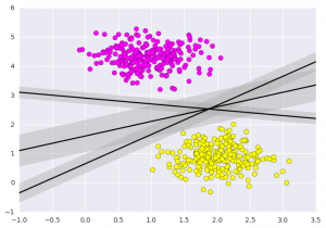
Output: 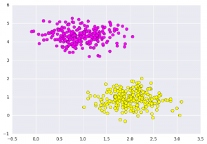What Support vector machines do, is to not only draw a line between two classes here, but consider a region about the line of some given width. Here’s an example of what it can look like: 

python3

# creating linspace between -1 to 3.5
xfit = np.linspace(-1, 3.5)

# plotting scatter
plt.scatter(X[:, 0], X[:, 1], c=Y, s=50, cmap='spring')

# plot a line between the different sets of data
for m, b, d in [(1, 0.65, 0.33), (0.5, 1.6, 0.55), (-0.2, 2.9, 0.2)]:
    yfit = m * xfit + b
    plt.plot(xfit, yfit, '-k')
    plt.fill_between(xfit, yfit - d, yfit + d, edgecolor='none',
    color='#AAAAAA', alpha=0.4)

plt.xlim(-1, 3.5);
plt.show()

Importing datasets

This is the intuition of support vector machines, which optimize a linear discriminant model representing the perpendicular distance between the datasets. Now let’s train the classifier using our training data. Before training, we need to import cancer datasets as csv file where we will train two features out of all features. 

python3

# importing required libraries
import numpy as np
import pandas as pd
import matplotlib.pyplot as plt

# reading csv file and extracting class column to y.
x = pd.read_csv("C:\...\cancer.csv")
a = np.array(x)
y  = a[:,30] # classes having 0 and 1

# extracting two features
x = np.column_stack((x.malignant,x.benign))

# 569 samples and 2 features
x.shape

print (x),(y)

[[  122.8   1001.  ]
 [  132.9   1326.  ]
 [  130.    1203.  ]
 ..., 
 [  108.3    858.1 ]
 [  140.1   1265.  ]
 [   47.92   181.  ]]

array([ 0.,  0.,  0.,  0.,  0.,  0.,  0.,  0.,  0.,  0.,  0.,  0.,  0.,
         0.,  0.,  0.,  0.,  0.,  0.,  1.,  1.,  1.,  0.,  0.,  0.,  0.,
         0.,  0.,  0.,  0.,  0.,  0.,  0.,  0.,  0.,  0.,  0.,  1.,  0.,
         0.,  0.,  0.,  0.,  0.,  0.,  0.,  1.,  0.,  1.,  1.,  1.,  1.,
         1.,  0.,  0.,  1.,  0.,  0.,  1.,  1.,  1.,  1.,  0.,  1., ....,
         1.])

Fitting a Support Vector Machine

Now we’ll fit a Support Vector Machine Classifier to these points. While the mathematical details of the likelihood model are interesting, we’ll let read about those elsewhere. Instead, we’ll just treat the scikit-learn algorithm as a black box which accomplishes the above task. 

python3

# import support vector classifier
# "Support Vector Classifier"
from sklearn.svm import SVC
clf = SVC(kernel='linear')

# fitting x samples and y classes
clf.fit(x, y)

After being fitted, the model can then be used to predict new values: 

python3

clf.predict([[120, 990]])

clf.predict([[85, 550]])

array([ 0.])
array([ 1.])

Let’s have a look on the graph how does this show. 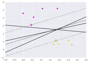This is obtained by analyzing the data taken and pre-processing methods to make optimal hyperplanes using matplotlib func If you like GeeksforGeeks and would like to contribute, you can also write an article using write.geeksforgeeks.org or mail your article to review-team@geeksforgeeks.org. See your article appearing on the GeeksforGeeks main page and help other Geeks.