Python | ARIMA Model for Time Series Forecasting

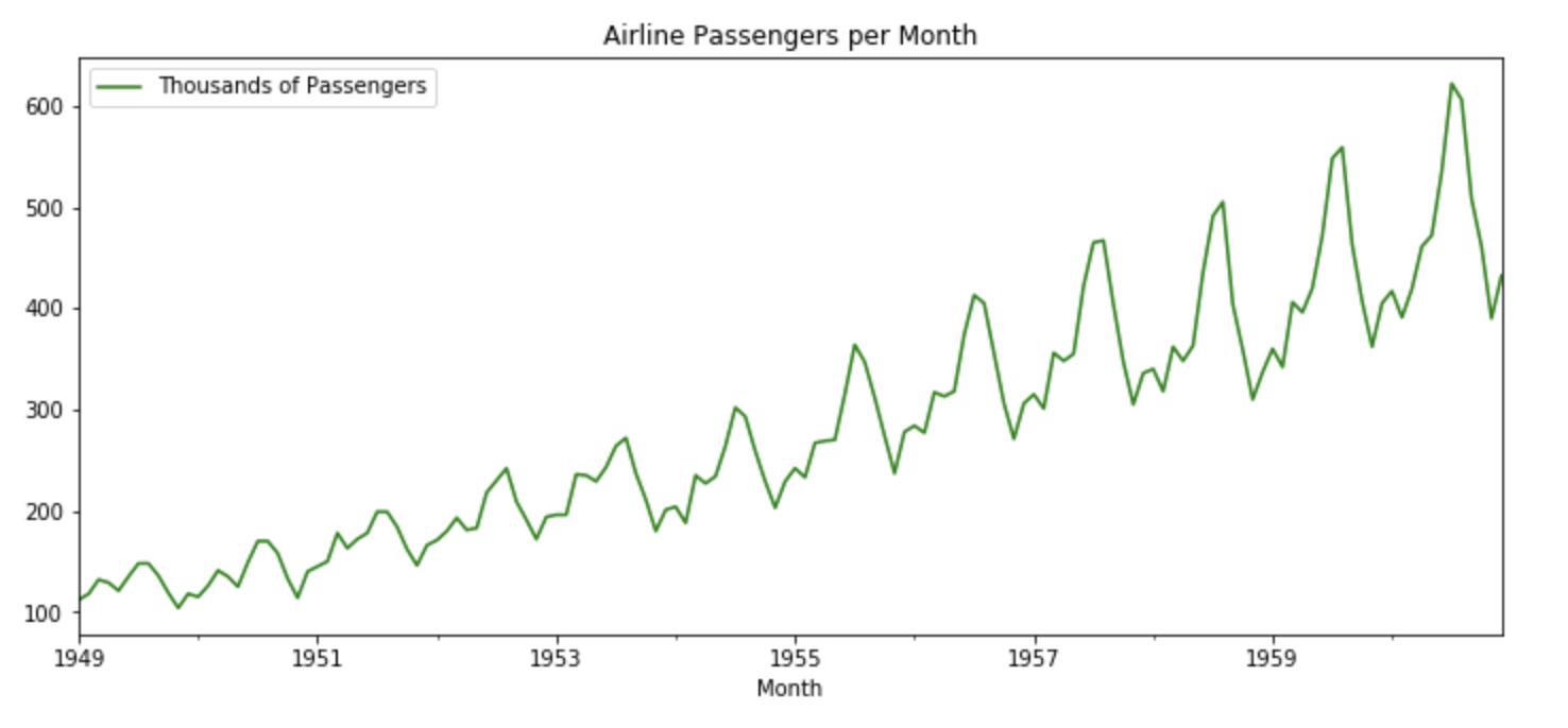
A Time Series is defined as a series of data points indexed in time order. The time order can be daily, monthly, or even yearly. Given below is an example of a Time Series that illustrates the number of passengers of an airline per month from the year 1949 to 1960.

Time Series Forecasting
Time Series forecasting is the process of using a statistical model to predict future values of a time series based on past results.

Some Use Cases

To predict the number of incoming or churning customers.

To explaining seasonal patterns in sales.

To detect unusual events and estimate the magnitude of their effect.

To Estimate the effect of a newly launched product on number of sold units.

Components of a Time Series:

• Trend:The trend shows a general direction of the time series data over a long period of time. A trend can be increasing(upward), decreasing(downward), or horizontal(stationary).
• Seasonality:The seasonality component exhibits a trend that repeats with respect to timing, direction, and magnitude. Some examples include an increase in water consumption in summer due to hot weather conditions, or an increase in the number of airline passengers during holidays each year.
• Cyclical Component: These are the trends with no set repetition over a particular period of time. A cycle refers to the period of ups and downs, booms and slums of a time series, mostly observed in business cycles. These cycles do not exhibit a seasonal variation but generally occur over a time period of 3 to 12 years depending on the nature of the time series.
• Irregular Variation: These are the fluctuations in the time series data which become evident when trend and cyclical variations are removed. These variations are unpredictable, erratic, and may or may not be random.
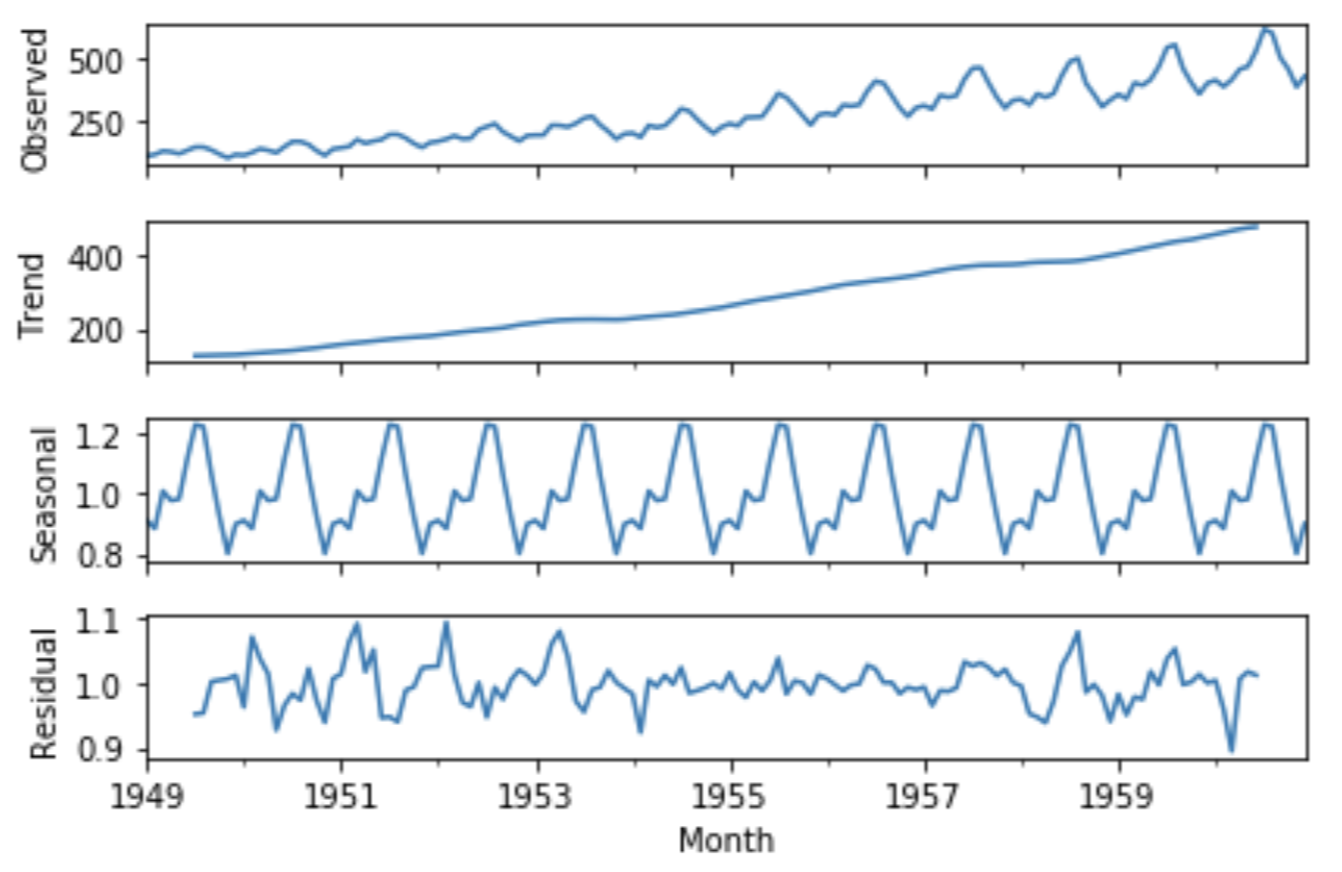
• ETS Decomposition
  ETS Decomposition is used to separate different components of a time series. The term ETS stands for Error, Trend, and Seasonality.

Code: ETS Decomposition of Airline Passengers Dataset:

# Importing required libraries
import numpy as np
import pandas as pd
import matplotlib.pylot as plt
from statsmodels.tsa.seasonal import seasonal_decompose

# Read the AirPassengers dataset
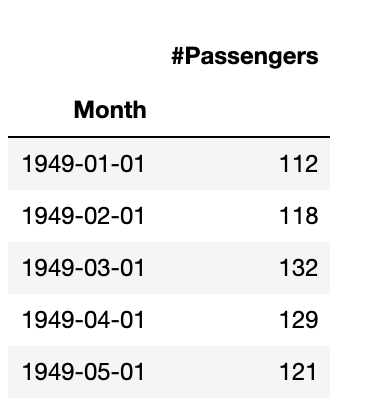
airline = pd.read_csv('AirPassengers.csv',
                       index_col ='Month',
                       parse_dates = True)

# Print the first five rows of the dataset
airline.head()

# ETS Decomposition
result = seasonal_decompose(airline['# Passengers'],
                            model ='multiplicative')

# ETS plot
result.plot()

Output:





ARIMA Model for Time Series Forecasting
ARIMA stands for autoregressive integrated moving average model and is specified by three order parameters: (p, d, q).

• AR(p) Autoregression – a regression model that utilizes the dependent relationship between a current observation and observations over a previous period.An auto regressive (AR(p)) component refers to the use of past values in the regression equation for the time series.
• I(d) Integration – uses differencing of observations (subtracting an observation from observation at the previous time step) in order to make the time series stationary. Differencing involves the subtraction of the current values of a series with its previous values d number of times.
• MA(q) Moving Average – a model that uses the dependency between an observation and a residual error from a moving average model applied to lagged observations. A moving average component depicts the error of the model as a combination of previous error terms. The order q represents the number of terms to be included in the model.

Types of ARIMA Model

• ARIMA:Non-seasonal Autoregressive Integrated Moving Averages
• SARIMA:Seasonal ARIMA
• SARIMAX:Seasonal ARIMA with exogenous variables

Pyramid Auto-ARIMA

The ‘auto_arima’ function from the ‘pmdarima’ library helps us to identify the most optimal parameters for an ARIMA model and returns a fitted ARIMA model.

Code : Parameter Analysis for the ARIMA model

# To install the library
pip install pmdarima

# Import the library
from pmdarima import auto_arima

# Ignore harmless warnings
import warnings
warnings.filterwarnings("ignore")

# Fit auto_arima function to AirPassengers dataset
stepwise_fit = auto_arima(airline['# Passengers'], start_p = 1, start_q = 1,
                          max_p = 3, max_q = 3, m = 12,
                          start_P = 0, seasonal = True,
                          d = None, D = 1, trace = True,
                          error_action ='ignore',   # we don't want to know if an order does not work
                          suppress_warnings = True,  # we don't want convergence warnings
                          stepwise = True)           # set to stepwise

# To print the summary
stepwise_fit.summary()

Output:


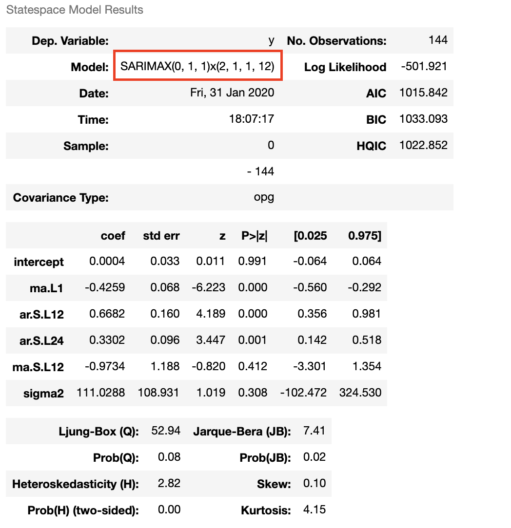
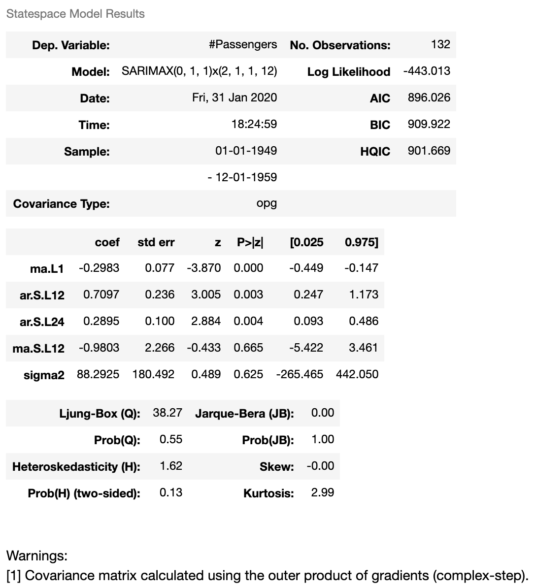
Code : Fit ARIMA Model to AirPassengers dataset

# Split data into train / test sets
train = airline.iloc[:len(airline)-12]
test = airline.iloc[len(airline)-12:] # set one year(12 months) for testing

# Fit a SARIMAX(0, 1, 1)x(2, 1, 1, 12) on the training set
from statsmodels.tsa.statespace.sarimax import SARIMAX

model = SARIMAX(train['# Passengers'],
                order = (0, 1, 1),
                seasonal_order =(2, 1, 1, 12))

result = model.fit()
result.summary()

Output:


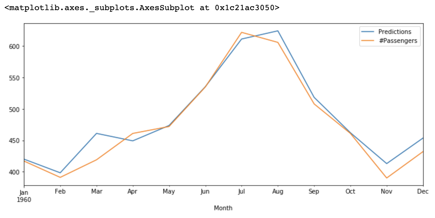
Code : Predictions of ARIMA Model against the test set

start = len(train)
end = len(train) + len(test) - 1

# Predictions for one-year against the test set
predictions = result.predict(start, end,
                             typ = 'levels').rename("Predictions")

# plot predictions and actual values
predictions.plot(legend = True)
test['# Passengers'].plot(legend = True)

Output:



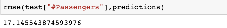
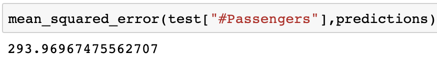
Code : Evaluate the model using MSE and RMSE

# Load specific evaluation tools
from sklearn.metrics import mean_squared_error
from statsmodels.tools.eval_measures import rmse

# Calculate root mean squared error
rmse(test["# Passengers"], predictions)

# Calculate mean squared error
mean_squared_error(test["# Passengers"], predictions)

Output:




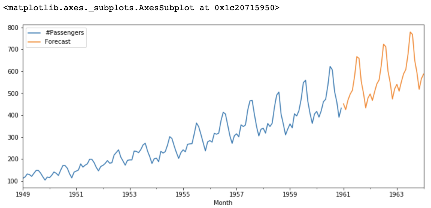
Code : Forecast using ARIMA Model

# Train the model on the full dataset
model = model = SARIMAX(airline['# Passengers'],
                        order = (0, 1, 1),
                        seasonal_order =(2, 1, 1, 12))
result = model.fit()

# Forecast for the next 3 years
forecast = result.predict(start = len(airline),
                          end = (len(airline)-1) + 3 * 12,
                          typ = 'levels').rename('Forecast')

# Plot the forecast values
airline['# Passengers'].plot(figsize = (12, 5), legend = True)
forecast.plot(legend = True)

Output: