Locally weighted linear Regression using Python

Locally weighted linear regression is the nonparametric regression methods that combine k-nearest neighbor based machine learning. It is referred to as locally weighted because for a query point the function is approximated on the basis of data near that and weighted because the contribution is weighted by its distance from the query point.

Locally Weighted Regression (LWR) is a non-parametric, memory-based algorithm, which means it explicitly retains training data and used it for every time a prediction is made.

To explain the locally weighted linear regression, we first need to understand the linear regression. The linear regression can be explained with the following equations:

Let (x_i, y_i) be the query point, then for minimizing the cost function in the linear regression:

by calculating  so, that it minimize the above cost function.

Our output will be: 

Thus, the formula for calculating \theta can also be:

where, beta is the vector of linear vector, X, Y is the matrix, and vector of all observations.

For locally weighted linear regression:

by calculating

so, that it minimize the above cost function.

Our output will be: 

Here, w(i) is the weight associated with each observation of training data. It can be calculated by the given formula:

Or this can be represented in the form of a matrix calculation:

Impact of Bandwidth

where x(i) is the observation from the training data and x is a particular point from which the distance is calculated and T(tau) is the bandwidth. Here, T(tau) decides the amount of fitness in the function, if the function is closely fitted, its value will be small. Therefore,

then, we can calculate \theta with the following equation:

Implementation

• For this implementation, we will be using bokeh. If you want to know bokeh functionalities in details please check this article

Python3

# Necessary imports
import numpy as np
from ipywidgets import interact
from bokeh.plotting import figure, show, output_notebook
from bokeh.layouts import gridplot
%matplotlib inline
output_notebook()
plt.style.use('seaborn-dark')

# function to perform locally weighted linear regression
def local_weighted_regression(x0, X, Y, tau):
    # add bias term
    x0 = np.r_[1, x0]
    X = np.c_[np.ones(len(X)), X]

    # fit model: normal equations with kernel
    xw = X.T * weights_calculate(x0, X, tau)
    theta = np.linalg.pinv(xw @ X) @ xw @ Y
    # "@" is used to
    # predict value
    return x0 @ theta

# function to perform weight calculation
def weights_calculate(x0, X, tau):
    return np.exp(np.sum((X - x0) ** 2, axis=1) / (-2 * (tau **2) ))

# plot locally weighted regression for different bandwidth values
def plot_lwr(tau):
    # prediction
    domain = np.linspace(-3, 3, num=300)
    prediction = [local_regression(x0, X, Y, tau) for x0 in domain]

    plot = figure(plot_width=400, plot_height=400)
    plot.title.text = 'tau=%g' % tau
    plot.scatter(X, Y, alpha=.3)
    plot.line(domain, prediction, line_width=2, color='red')

    return plot

#define distribution
n = 1000

# generate dataset
X = np.linspace(-3, 3, num=n)
Y = np.abs(X ** 3 - 1)

# jitter X
X += np.random.normal(scale=.1, size=n)

# show the plots for different values of Tau
show(gridplot([
    [plot_lwr(10.), plot_lwr(1.)],
    [plot_lwr(0.1), plot_lwr(0.01)]
]))

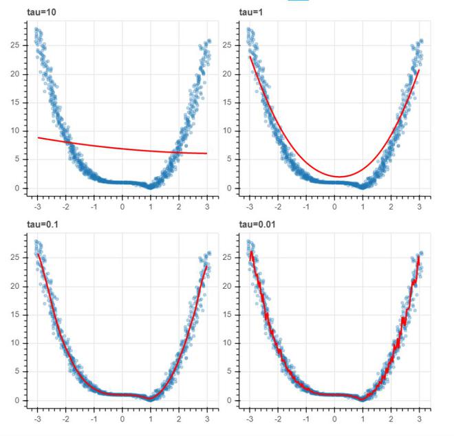
LWR plot with different values of bandwidth

• As we can notice from the above plot that with small values of bandwidth, the model fits better but sometimes it will lead to overfitting.

References:

• Stanford CS 229