Data cleaning is one of the important parts of machine learning. It plays a significant part in building a model. In this article, we’ll understand Data cleaning, its significance and Python implementation.
What is Data Cleaning?
Data cleaning is a crucial step in the machine learning (ML) pipeline, as it involves identifying and removing any missing, duplicate, or irrelevant data. The goal of data cleaning is to ensure that the data is accurate, consistent, and free of errors, as incorrect or inconsistent data can negatively impact the performance of the ML model. Professional data scientists usually invest a very large portion of their time in this step because of the belief that “Better data beats fancier algorithms”.
Data cleaning, also known as data cleansing or data preprocessing, is a crucial step in the data science pipeline that involves identifying and correcting or removing errors, inconsistencies, and inaccuracies in the data to improve its quality and usability. Data cleaning is essential because raw data is often noisy, incomplete, and inconsistent, which can negatively impact the accuracy and reliability of the insights derived from it.
Why is Data Cleaning Important?
Data cleansing is a crucial step in the data preparation process, playing an important role in ensuring the accuracy, reliability, and overall quality of a dataset.
For decision-making, the integrity of the conclusions drawn heavily relies on the cleanliness of the underlying data. Without proper data cleaning, inaccuracies, outliers, missing values, and inconsistencies can compromise the validity of analytical results. Moreover, clean data facilitates more effective modeling and pattern recognition, as algorithms perform optimally when fed high-quality, error-free input.
Additionally, clean datasets enhance the interpretability of findings, aiding in the formulation of actionable insights.
Data Cleaning in Data Science
Data clean-up is an integral component of data science, playing a fundamental role in ensuring the accuracy and reliability of datasets. In the field of data science, where insights and predictions are drawn from vast and complex datasets, the quality of the input data significantly influences the validity of analytical results. Data cleaning involves the systematic identification and correction of errors, inconsistencies, and inaccuracies within a dataset, encompassing tasks such as handling missing values, removing duplicates, and addressing outliers. This meticulous process is essential for enhancing the integrity of analyses, promoting more accurate modeling, and ultimately facilitating informed decision-making based on trustworthy and high-quality data.
Steps to Perform Data Cleanliness
Performing data cleaning involves a systematic process to identify and rectify errors, inconsistencies, and inaccuracies in a dataset. The following are essential steps to perform data cleaning.
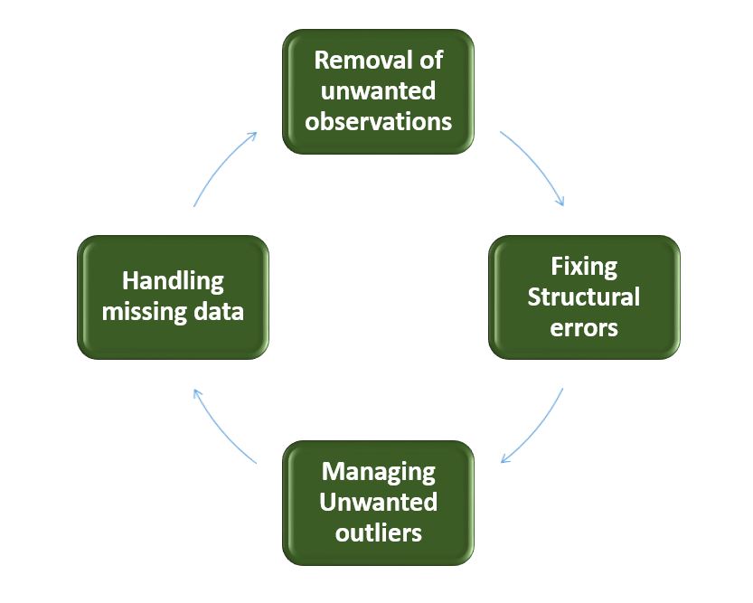
Data Cleaning
- Removal of Unwanted Observations: Identify and eliminate irrelevant or redundant observations from the dataset. The step involves scrutinizing data entries for duplicate records, irrelevant information, or data points that do not contribute meaningfully to the analysis. Removing unwanted observations streamlines the dataset, reducing noise and improving the overall quality.
- Fixing Structure errors: Address structural issues in the dataset, such as inconsistencies in data formats, naming conventions, or variable types. Standardize formats, correct naming discrepancies, and ensure uniformity in data representation. Fixing structure errors enhances data consistency and facilitates accurate analysis and interpretation.
- Managing Unwanted outliers: Identify and manage outliers, which are data points significantly deviating from the norm. Depending on the context, decide whether to remove outliers or transform them to minimize their impact on analysis. Managing outliers is crucial for obtaining more accurate and reliable insights from the data.
- Handling Missing Data: Devise strategies to handle missing data effectively. This may involve imputing missing values based on statistical methods, removing records with missing values, or employing advanced imputation techniques. Handling missing data ensures a more complete dataset, preventing biases and maintaining the integrity of analyses.
How to Perform Data Cleanliness
Performing data cleansing involves a systematic approach to enhance the quality and reliability of a dataset. The process begins with a thorough understanding of the data, inspecting its structure and identifying issues such as missing values, duplicates, and outliers. Addressing missing data involves strategic decisions on imputation or removal, while duplicates are systematically eliminated to reduce redundancy. Managing outliers ensures that extreme values do not unduly influence analysis. Structural errors are corrected to standardize formats and variable types, promoting consistency.
Throughout the process, documentation of changes is crucial for transparency and reproducibility. Iterative validation and testing confirm the effectiveness of the data cleansing steps, ultimately resulting in a refined dataset ready for meaningful analysis and insights.
Python Implementation for Database Cleaning
Let’s understand each step for Database Cleaning, using titanic dataset. Below are the necessary steps:
- Import the necessary libraries
- Load the dataset
- Check the data information using df.info()
Python3
import pandas as pd
import numpy as np
df = pd.read_csv('titanic.csv')
df.head()
|
Output:
PassengerId    Survived    Pclass    Name    Sex    Age    SibSp    Parch    Ticket    Fare    Cabin    Embarked
0    1    0    3    Braund, Mr. Owen Harris    male    22.0    1    0    A/5 21171    7.2500    NaN    S
1    2    1    1    Cumings, Mrs. John Bradley (Florence Briggs Th...    female    38.0    1    0    PC 17599    71.2833    C85    C
2    3    1    3    Heikkinen, Miss. Laina    female    26.0    0    0    STON/O2. 3101282    7.9250    NaN    S
3    4    1    1    Futrelle, Mrs. Jacques Heath (Lily May Peel)    female    35.0    1    0    113803    53.1000    C123    S
4    5    0    3    Allen, Mr. William Henry    male    35.0    0    0    373450    8.0500    NaN    S
Data Inspection and Exploration
Let’s first understand the data by inspecting its structure and identifying missing values, outliers, and inconsistencies and check the duplicate rows with below python code:
Output:
0      False
1      False
2      False
3      False
4      False
       ...
886    False
887    False
888    False
889    False
890    False
Length: 891, dtype: bool
Check the data information using df.info()
Output:
<class 'pandas.core.frame.DataFrame'>
RangeIndex: 891 entries, 0 to 890
Data columns (total 12 columns):
 #   Column       Non-Null Count  Dtype
---  ------       --------------  -----
 0   PassengerId  891 non-null    int64
 1   Survived     891 non-null    int64
 2   Pclass       891 non-null    int64
 3   Name         891 non-null    object
 4   Sex          891 non-null    object
 5   Age          714 non-null    float64
 6   SibSp        891 non-null    int64
 7   Parch        891 non-null    int64
 8   Ticket       891 non-null    object
 9   Fare         891 non-null    float64
 10  Cabin        204 non-null    object
 11  Embarked     889 non-null    object
dtypes: float64(2), int64(5), object(5)
memory usage: 83.7+ KB
From the above data info, we can see that Age and Cabin have an unequal number of counts. And some of the columns are categorical and have data type objects and some are integer and float values.
Check the Categorical and Numerical Columns.
Python3
cat_col = [col for col in df.columns if df[col].dtype == 'object']
print('Categorical columns :',cat_col)
num_col = [col for col in df.columns if df[col].dtype != 'object']
print('Numerical columns :',num_col)
|
Output:
Categorical columns : ['Name', 'Sex', 'Ticket', 'Cabin', 'Embarked']
Numerical columns : ['PassengerId', 'Survived', 'Pclass', 'Age', 'SibSp', 'Parch', 'Fare']
Check the total number of Unique Values in the Categorical Columns
Output:
Name        891
Sex           2
Ticket      681
Cabin       147
Embarked      3
dtype: int64
Steps to Perform Data Cleansing
Removal of all Above Unwanted Observations
This includes deleting duplicate/ redundant or irrelevant values from your dataset. Duplicate observations most frequently arise during data collection and Irrelevant observations are those that don’t actually fit the specific problem that you’re trying to solve.
- Redundant observations alter the efficiency to a great extent as the data repeats and may add towards the correct side or towards the incorrect side, thereby producing unfaithful results.
- Irrelevant observations are any type of data that is of no use to us and can be removed directly.
Now we have to make a decision according to the subject of analysis, which factor is important for our discussion.
As we know our machines don’t understand the text data. So, we have to either drop or convert the categorical column values into numerical types. Here we are dropping the Name columns because the Name will be always unique and it hasn’t a great influence on target variables. For the ticket, Let’s first print the 50 unique tickets.
Python3
df['Ticket'].unique()[:50]
|
Output:
array(['A/5 21171', 'PC 17599', 'STON/O2. 3101282', '113803', '373450',
       '330877', '17463', '349909', '347742', '237736', 'PP 9549',
       '113783', 'A/5. 2151', '347082', '350406', '248706', '382652',
       '244373', '345763', '2649', '239865', '248698', '330923', '113788',
       '347077', '2631', '19950', '330959', '349216', 'PC 17601',
       'PC 17569', '335677', 'C.A. 24579', 'PC 17604', '113789', '2677',
       'A./5. 2152', '345764', '2651', '7546', '11668', '349253',
       'SC/Paris 2123', '330958', 'S.C./A.4. 23567', '370371', '14311',
       '2662', '349237', '3101295'], dtype=object)
From the above tickets, we can observe that it is made of two like first values ‘A/5 21171’ is joint from of ‘A/5’ and ‘21171’ this may influence our target variables. It will the case of Feature Engineering. where we derived new features from a column or a group of columns. In the current case, we are dropping the “Name” and “Ticket” columns.
Drop Name and Ticket Columns
Python3
df1 = df.drop(columns=['Name','Ticket'])
df1.shape
|
Output:
(891, 10)
Handling Missing Data
Missing data is a common issue in real-world datasets, and it can occur due to various reasons such as human errors, system failures, or data collection issues. Various techniques can be used to handle missing data, such as imputation, deletion, or substitution.
Let’s check the % missing values columns-wise for each row using df.isnull() it checks whether the values are null or not and gives returns boolean values. and .sum() will sum the total number of null values rows and we divide it by the total number of rows present in the dataset then we multiply to get values in % i.e per 100 values how much values are null.
Python3
round((df1.isnull().sum()/df1.shape[0])*100,2)
|
Output:
PassengerId     0.00
Survived        0.00
Pclass          0.00
Sex             0.00
Age            19.87
SibSp           0.00
Parch           0.00
Fare            0.00
Cabin          77.10
Embarked        0.22
dtype: float64
We cannot just ignore or remove the missing observation. They must be handled carefully as they can be an indication of something important.
The two most common ways to deal with missing data are:
- Dropping Observations with missing values.
- The fact that the value was missing may be informative in itself.
- Plus, in the real world, you often need to make predictions on new data even if some of the features are missing!
As we can see from the above result that Cabin has 77% null values and Age has 19.87% and Embarked has 0.22% of null values.
So, it’s not a good idea to fill 77% of null values. So, we will drop the Cabin column. Embarked column has only 0.22% of null values so, we drop the null values rows of Embarked column.
Python3
df2 = df1.drop(columns='Cabin')
df2.dropna(subset=['Embarked'], axis=0, inplace=True)
df2.shape
|
Output:
(889, 9)
- Imputing the missing values from past observations.
- Again, “missingness” is almost always informative in itself, and you should tell your algorithm if a value was missing.
- Even if you build a model to impute your values, you’re not adding any real information. You’re just reinforcing the patterns already provided by other features.
We can use Mean imputation or Median imputations for the case.
Note:
- Mean imputation is suitable when the data is normally distributed and has no extreme outliers.
- Median imputation is preferable when the data contains outliers or is skewed.
Python3
df3 = df2.fillna(df2.Age.mean())
df3.isnull().sum()
|
Output:
PassengerId    0
Survived       0
Pclass         0
Sex            0
Age            0
SibSp          0
Parch          0
Fare           0
Embarked       0
dtype: int64
Handling Outliers
Outliers are extreme values that deviate significantly from the majority of the data. They can negatively impact the analysis and model performance. Techniques such as clustering, interpolation, or transformation can be used to handle outliers.
To check the outliers, We generally use a box plot. A box plot, also referred to as a box-and-whisker plot, is a graphical representation of a dataset’s distribution. It shows a variable’s median, quartiles, and potential outliers. The line inside the box denotes the median, while the box itself denotes the interquartile range (IQR). The whiskers extend to the most extreme non-outlier values within 1.5 times the IQR. Individual points beyond the whiskers are considered potential outliers. A box plot offers an easy-to-understand overview of the range of the data and makes it possible to identify outliers or skewness in the distribution.
Let’s plot the box plot for Age column data.
Python3
import matplotlib.pyplot as plt
plt.boxplot(df3['Age'], vert=False)
plt.ylabel('Variable')
plt.xlabel('Age')
plt.title('Box Plot')
plt.show()
|
Output:
.png)
Box Plot
As we can see from the above Box and whisker plot, Our age dataset has outliers values. The values less than 5 and more than 55 are outliers.
Python3
mean = df3['Age'].mean()
std = df3['Age'].std()
lower_bound = mean - std*2
upper_bound = mean + std*2
print('Lower Bound :',lower_bound)
print('Upper Bound :',upper_bound)
df4 = df3[(df3['Age'] >= lower_bound)
& (df3['Age'] <= upper_bound)]
|
Output:
Lower Bound : 3.705400107925648
Upper Bound : 55.578785285332785
Similarly, we can remove the outliers of the remaining columns.
Data Transformation
Data transformation involves converting the data from one form to another to make it more suitable for analysis. Techniques such as normalization, scaling, or encoding can be used to transform the data.
Data validation and verification
Data validation and verification involve ensuring that the data is accurate and consistent by comparing it with external sources or expert knowledge.
For the machine learning prediction, First, we separate independent and target features. Here we will consider only ‘Sex’ ‘Age’ ‘SibSp’, ‘Parch’ ‘Fare’ ‘Embarked’ only as the independent features and Survived as target variables. Because PassengerId will not affect the survival rate.
Python3
X = df3[['Pclass','Sex','Age', 'SibSp','Parch','Fare','Embarked']]
Y = df3['Survived']
|
Data formatting
Data formatting involves converting the data into a standard format or structure that can be easily processed by the algorithms or models used for analysis. Here we will discuss commonly used data formatting techniques i.e. Scaling and Normalization.
Scaling
- Scaling involves transforming the values of features to a specific range. It maintains the shape of the original distribution while changing the scale.
- Particularly useful when features have different scales, and certain algorithms are sensitive to the magnitude of the features.
- Common scaling methods include Min-Max scaling and Standardization (Z-score scaling).
Min-Max Scaling: Min-Max scaling rescales the values to a specified range, typically between 0 and 1. It preserves the original distribution and ensures that the minimum value maps to 0 and the maximum value maps to 1.
Python3
from sklearn.preprocessing import MinMaxScaler
scaler = MinMaxScaler(feature_range=(0, 1))
num_col_ = [col for col in X.columns if X[col].dtype != 'object']
x1 = X
x1[num_col_] = scaler.fit_transform(x1[num_col_])
x1.head()
|
Output:
Pclass    Sex    Age    SibSp    Parch    Fare    Embarked
0    1.0    male    0.271174    0.125    0.0    0.014151    S
1    0.0    female    0.472229    0.125    0.0    0.139136    C
2    1.0    female    0.321438    0.000    0.0    0.015469    S
3    0.0    female    0.434531    0.125    0.0    0.103644    S
4    1.0    male    0.434531    0.000    0.0    0.015713    S
Standardization (Z-score scaling): Standardization transforms the values to have a mean of 0 and a standard deviation of 1. It centers the data around the mean and scales it based on the standard deviation. Standardization makes the data more suitable for algorithms that assume a Gaussian distribution or require features to have zero mean and unit variance.
Z = (X - μ) / σ
Where,
- X = Data
- μ = Mean value of X
- σ = Standard deviation of X
Data Cleansing Tools
Some data cleansing tools:
- OpenRefine
- Trifacta Wrangler
- TIBCO Clarity
- Cloudingo
- IBM Infosphere Quality Stage
Advantages of Data Cleaning in Machine Learning:
- Improved model performance: Removal of errors, inconsistencies, and irrelevant data, helps the model to better learn from the data.
- Increased accuracy: Helps ensure that the data is accurate, consistent, and free of errors.
- Better representation of the data: Data cleaning allows the data to be transformed into a format that better represents the underlying relationships and patterns in the data.
- Improved data quality: Improve the quality of the data, making it more reliable and accurate.
- Improved data security: Helps to identify and remove sensitive or confidential information that could compromise data security.
Disadvantages of Data Cleaning in Machine Learning
- Time-consuming: Time-Consuming task, especially for large and complex datasets.
- Error-prone: Data cleaning can be error-prone, as it involves transforming and cleaning the data, which can result in the loss of important information or the introduction of new errors.
- Cost and resource-intensive: Resource-intensive process that requires significant time, effort, and expertise. It can also require the use of specialized software tools, which can add to the cost and complexity of data cleaning.
- Overfitting: Data cleaning can inadvertently contribute to overfitting by removing too much data.
Conclusion
So, we have discussed four different steps in data cleaning to make the data more reliable and to produce good results. After properly completing the Data Cleaning steps, we’ll have a robust dataset that avoids many of the most common pitfalls. In summary, data cleaning is a crucial step in the data science pipeline that involves identifying and correcting errors, inconsistencies, and inaccuracies in the data to improve its quality and usability.
What is Data Cleansing- FAQs
What does it mean to cleanse our data?
Cleansing data involves identifying and rectifying errors, inconsistencies, and inaccuracies in a dataset to improve its quality, ensuring reliable results in analyses and decision-making.
What is an example of cleaning data?
Removing duplicate records in a customer database ensures accurate and unbiased analysis, preventing redundant information from skewing results or misrepresenting the customer base.
What is the meaning of data wash?
“Data wash” is not a standard term in data management. If used, it could refer to cleaning or processing data, but it’s not a widely recognized term in the field.
How is data cleansing done?
Data cleansing involves steps like removing duplicates, handling missing values, and correcting inconsistencies. It requires systematic examination and correction of data issues.
What is data cleansing in cyber security?
In cybersecurity, data cleansing involves identifying and removing malicious code or unauthorized access points from datasets to protect sensitive information and prevent cyber threats.
How to clean data using SQL?
Use SQL commands like DELETE for removing duplicates, UPDATE for correcting values, and ALTER TABLE for modifying data structures. Employ WHERE clauses to target specific records for cleaning.
Like Article
Suggest improvement
Share your thoughts in the comments
Please Login to comment...