ML – Gradient Boosting

Gradient Boosting is a popular boosting algorithm. In gradient boosting, each predictor corrects its predecessor’s error. In contrast to Adaboost, the weights of the training instances are not tweaked, instead, each predictor is trained using the residual errors of predecessor as labels.

There is a technique called the Gradient Boosted Trees whose base learner is CART (Classification and Regression Trees).

The below diagram explains how gradient boosted trees are trained for regression problems.

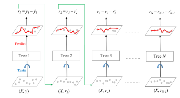
Gradient Boosted Trees for Regression

The ensemble consists of N trees. Tree1 is trained using the feature matrix X and the labels y. The predictions labelled y1(hat) are used to determine the training set residual errors r1. Tree2 is then trained using the feature matrix X and the residual errors r1 of Tree1 as labels. The predicted results r1(hat) are then used to determine the residual r2. The process is repeated until all the N trees forming the ensemble are trained.

There is an important parameter used in this technique known as Shrinkage.

Shrinkage refers to the fact that the prediction of each tree in the ensemble is shrunk after it is multiplied by the learning rate (eta) which ranges between 0 to 1. There is a trade-off between eta and number of estimators, decreasing learning rate needs to be compensated with increasing estimators in order to reach certain model performance. Since all trees are trained now, predictions can be made.

Each tree predicts a label and final prediction is given by the formula,

y(pred) = y1 + (eta *  r1) + (eta * r2) + ....... + (eta * rN)

The class of the gradient boosting regression in scikit-learn is GradientBoostingRegressor. A similar algorithm is used for classification known as GradientBoostingClassifier.

Code: Python code for Gradient Boosting Regressor

# Import models and utility functions
from sklearn.ensemble import GradientBoostingRegressor
from sklearn.model_selection import train_test_split
from sklearn.metrics import mean_squared_error as MSE
from sklearn import datasets

# Setting SEED for reproducibility
SEED = 1

# Importing the dataset
bike = datasets.load_bike()
X, y = bike.data, bike.target

# Splitting dataset
train_X, test_X, train_y, test_y = train_test_split(X, y, test_size = 0.3, random_state = SEED)

# Instantiate Gradient Boosting Regressor
gbr = GradientBoostingRegressor(n_estimators = 200, max_depth = 1, random_state = SEED)

# Fit to training set
gbr.fit(train_X, train_y)

# Predict on test set
pred_y = gbr.predict(test_X)

# test set RMSE
test_rmse = MSE(test_y, pred_y) ** (1 / 2)

# Print rmse
print('RMSE test set: {:.2f}'.format(test_rmse))

Output:

RMSE test set: 4.01

My Personal Notes arrow_drop_up

Save