Time Series Analysis in R

Time Series Analysis in R is used to see how an object behaves over a period of time. In R Programming Language, it can be easily done by the ts() function with some parameters. Time series takes the data vector and each data is connected with a timestamp value as given by the user. This function is mostly used to learn and forecast the behavior of an asset in business for a period of time. For example, sales analysis of a company, inventory analysis, price analysis of a particular stock or market, population analysis, etc.

Syntax:  objectName <- ts(data, start, end, frequency)

where,

• data – represents the data vector
• start – represents the first observation in time series
• end – represents the last observation in time series
• frequency – represents number of observations per unit time. For example, frequency=1 for monthly data.

Note: To know about more optional parameters, use the following command in the R console: 

help("ts")

Examples of Time Series Analysis

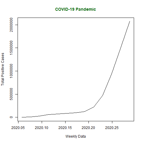
Let’s take the example of the COVID-19 pandemic situation. Taking the total number of positive cases of COVID-19 cases weekly from 22 January 2020 to 15 April 2020 the world in data vector.

R

# Weekly data of COVID-19 positive cases from
# 22 January, 2020 to 15 April, 2020
x <- c(580, 7813, 28266, 59287, 75700,
    87820, 95314, 126214, 218843, 471497,
    936851, 1508725, 2072113)

# library required for decimal_date() function
library(lubridate)

# output to be created as png file
png(file ="timeSeries.png")

# creating time series object
# from date 22 January, 2020
mts <- ts(x, start = decimal_date(ymd("2020-01-22")),
                            frequency = 365.25 / 7)

# plotting the graph
plot(mts, xlab ="Weekly Data",
        ylab ="Total Positive Cases",
        main ="COVID-19 Pandemic",
        col.main ="darkgreen")

# saving the file
dev.off()

Output:

Time Series Data visualization chart

Multivariate Time Series Analysis

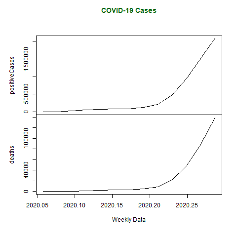
Multivariate Time Series is creating multiple time series in a single chart. Taking data of total positive cases and total deaths from COVID-19 weekly from 22 January 2020 to 15 April 2020 in a data vector. 

R

# Weekly data of COVID-19 positive cases and
# weekly deaths from 22 January, 2020 to
# 15 April, 2020

positiveCases <- c(580, 7813, 28266, 59287,
                75700, 87820, 95314, 126214,
                218843, 471497, 936851,
                1508725, 2072113)

deaths <- c(17, 270, 565, 1261, 2126, 2800,
            3285, 4628, 8951, 21283, 47210,
            88480, 138475)

# library required for decimal_date() function
library(lubridate)

# output to be created as png file
png(file="multivariateTimeSeries.png")

# creating multivariate time series object
# from date 22 January, 2020
mts <- ts(cbind(positiveCases, deaths),
start = decimal_date(ymd("2020-01-22")),
                    frequency = 365.25 / 7)

# plotting the graph
plot(mts, xlab ="Weekly Data",
    main ="COVID-19 Cases",
    col.main ="darkgreen")

# saving the file
dev.off()

Output:

Multivariate Time Series Analysis using R

Time Series Forecasting

Forecasting can be done on time series using some models present in R. In this example, Arima automated model is used. To know about more parameters of arima() function, use the below command. 

help("arima")

In the below code, forecasting is done using the forecast library and so, installation of the forecast library is necessary. 

R

# Weekly data of COVID-19 cases from
# 22 January, 2020 to 15 April, 2020
x <- c(580, 7813, 28266, 59287, 75700,
    87820, 95314, 126214, 218843,
    471497, 936851, 1508725, 2072113)

# library required for decimal_date() function
library(lubridate)

# library required for forecasting
library(forecast)

# output to be created as png file
png(file ="forecastTimeSeries.png")

# creating time series object
# from date 22 January, 2020
mts <- ts(x, start = decimal_date(ymd("2020-01-22")),
                            frequency = 365.25 / 7)

# forecasting model using arima model
fit <- auto.arima(mts)

# Next 5 forecasted values
forecast(fit, 5)

# plotting the graph with next
# 5 weekly forecasted values
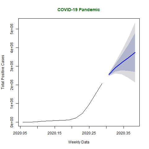
plot(forecast(fit, 5), xlab ="Weekly Data",
ylab ="Total Positive Cases",
main ="COVID-19 Pandemic", col.main ="darkgreen")

# saving the file
dev.off()

Output :

         Point Forecast   Lo 80   Hi 80   Lo 95   Hi 95
2020.307        2547989 2491957 2604020 2462296 2633682
2020.326        2915130 2721277 3108983 2618657 3211603
2020.345        3202354 2783402 3621307 2561622 3843087
2020.364        3462692 2748533 4176851 2370480 4554904
2020.383        3745054 2692884 4797225 2135898 5354210

Below graph plots estimated forecasted values of COVID-19 if it continues to be widespread for the next 5 weeks. 

Time Series Forecasting using R