In statistics, skewness and kurtosis are the measures that tell about the shape of the data distribution, or simply, both are numerical methods to analyze the shape of data set unlike, plotting graphs and histograms which are graphical methods. These are normality tests to check the irregularity and asymmetry of the distribution.
To calculate skewness and kurtosis in R language, a moments package is required.
Skewness
Skewness is a statistical numerical method to measure the asymmetry of the distribution or data set. It tells about the position of the majority of data values in the distribution around the mean value. A fundamental statistical notion called skewness quantifies the asymmetries in data distributions. It is essential to a number of disciplines, including data analysis, social sciences, economics, and finance.
Formula:

where,
represents coefficient of skewness
*** QuickLaTeX cannot compile formula:


*** Error message:
Error: Nothing to show, formula is empty
represents  value in data vector
*** QuickLaTeX cannot compile formula:


*** Error message:
Error: Nothing to show, formula is empty
represents mean of data vector
n represents total number of observations
There exist 3 types of skewness values on the basis of which the asymmetry of the graph is decided. These are as follows:
Positive Skew
The asymmetry of data distributions where the tail extends towards higher values is known statistically as positive skewness. It is a crucial metric in a number of disciplines, including data analysis, social sciences, finance, and economics. The definition, computation techniques, interpretation, and applications of positive skewness theory are covered in detail in this article.
If the coefficient of skewness is greater than 0 i.e. \gamma_{1}>0 , then the graph is said to be positively skewed with the majority of data values less than the mean. Most of the values are concentrated on the left side of the graph.
Example:
R
library(moments)
x <- c(40, 41, 42, 43, 50)
png(file = "positiveskew.png")
print(skewness(x))
hist(x)
dev.off()
|
Output:
[1] 1.2099
Graphical Representation:
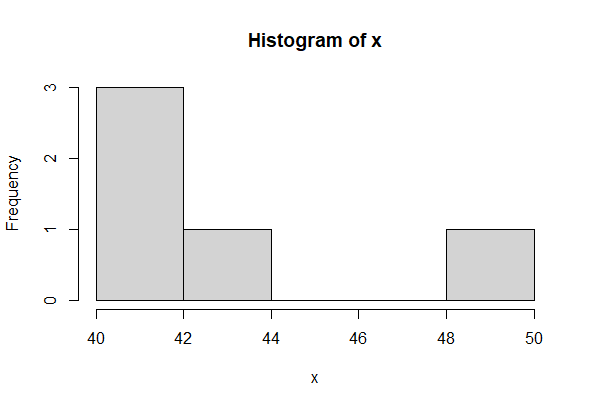
Simple Histogram
Zero Skewness or Symmetric
A statistical notion called zero skewness, commonly referred to as symmetry, defines data distributions that are balanced and have equal probability on both sides of the mean. It is a fundamental metric used in many disciplines, such as data analysis, economics, social sciences, and finance.
If the coefficient of skewness is equal to 0 or approximately close to 0 i.e.  , then the graph is said to be symmetric and data is normally distributed.
Example:
R
library(moments)
x <- rnorm(50, 10, 10)
png(file = "zeroskewness.png")
print(skewness(x))
hist(x)
dev.off()
|
Output:
[1] -0.02991511
Graphical Representation:
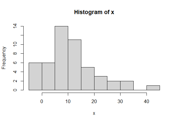
Simple Histogram
Negatively skewed
Left-skewed distributions, commonly referred to as negatively skewed distributions, are statistical notions that describe asymmetrical data distributions with a tail that slopes downward. In a number of disciplines, including finance, economics, social sciences, and data analysis, it is crucial to comprehend negatively skewed data.
If the coefficient of skewness is less than 0 i.e. \gamma_{1}<0 , then the graph is said to be negatively skewed with the majority of data values greater than the mean. Most of the values are concentrated on the right side of the graph.
Example:
R
library(moments)
x <- c(10, 11, 21, 22, 23, 25)
png(file = "negativeskew.png")
print(skewness(x))
hist(x)
dev.off()
|
Output:
[1] -0.5794294
Graphical Representation:
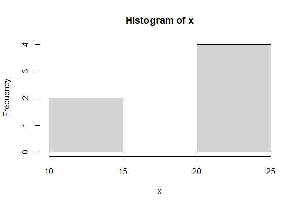
Simple Histogram
Kurtosis
A statistical measure known as kurtosis measures the peakedness, flatness, and weight of the tails of data distributions. In a number of disciplines, including finance, economics, social sciences, and data analysis, an understanding of kurtosis is crucial. Kurtosis theory is thoroughly explained in this article, which also covers its definition, computation processes, interpretation, and applications.
Kurtosis is a numerical method in statistics that measures the sharpness of the peak in the data distribution.
Formula:

where,
*** QuickLaTeX cannot compile formula:


*** Error message:
Error: Nothing to show, formula is empty
represents coefficient of kurtosis
*** QuickLaTeX cannot compile formula:


*** Error message:
Error: Nothing to show, formula is empty
represents value in data vector
*** QuickLaTeX cannot compile formula:


*** Error message:
Error: Nothing to show, formula is empty
represents mean of data vector
n represents total number of observations
There exist 3 types of Kurtosis values on the basis of which the sharpness of the peak is measured. These are as follows:
Platykurtic
Data distributions having flattened tails compared to the normal distribution are referred to statistically as platykurtic distributions. In several disciplines, including finance, economics, social sciences, and data analysis, it is essential to comprehend platykurtic data. The definition, calculation procedures, interpretation, and applications of Platykurtic.
If the coefficient of kurtosis is less than 3 i.e.  , then the data distribution is platykurtic. Being platykurtic doesn’t mean that the graph is flat-topped.
Example:
R
library(moments)
x <- c(rep(61, each = 10), rep(64, each = 18),
rep(65, each = 23), rep(67, each = 32), rep(70, each = 27),
rep(73, each = 17))
png(file = "platykurtic.png")
print(kurtosis(x))
hist(x)
dev.off()
|
Output:
[1] 2.258318
Graphical Representation:
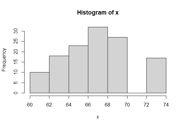
Histogram
Mesokurtic
Data distributions with tails that are similar in thickness to the normal distribution are known statistically as mesokurtic distributions. Numerous professions, including finance, economics, social sciences, and data analysis, depend on an understanding of mesokurtic data.
If the coefficient of kurtosis is equal to 3 or approximately close to 3 i.e. \gamma_{2}=3 , then the data distribution is mesokurtic. For the normal distribution, the kurtosis value is approximately equal to 3.
Example:
R
library(moments)
x <- rnorm(100)
png(file = "mesokurtic.png")
print(kurtosis(x))
hist(x)
dev.off()
|
Output:
[1] 2.963836
Graphical Representation:
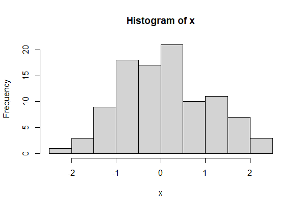
Histogram
Leptokurtic
Data distributions having hefty tails compared to the normal distribution are referred to statistically as leptokurtic distributions. In several disciplines, including finance, economics, social sciences, and data analysis, it is essential to comprehend leptokurtic data. The leptokurtic theory is thoroughly discussed in this article, including its concept, calculation techniques, interpretation, and applications.
If the coefficient of kurtosis is greater than 3 i.e.  , then the data distribution is leptokurtic and shows a sharp peak on the graph.
Example:
R
library(moments)
x <- c(rep(61, each = 2), rep(64, each = 5),
rep(65, each = 42), rep(67, each = 12), rep(70, each = 10))
png(file = "leptokurtic.png")
print(kurtosis(x))
hist(x)
dev.off()
|
Output:
[1] 3.696788
Graphical Representation:
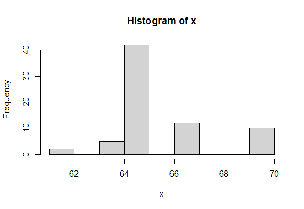
Histogram
Share your thoughts in the comments
Please Login to comment...