Time Series Analysis using Facebook Prophet in R Programming

Time Series Analysis is a way of analysing and learning the behaviour of datasets over a period. Moreover, it helps in learning the behavior of the dataset by plotting the time series object on the graph. In R programming, it can be easily performed by using ts() function that takes the data vector and converts it into time series object as specified in function parameters. Facebook Prophet is a tool developed by Facebook for forecasting time series objects or data. It helps businesses to learn the behavior of their products by forecasting prices, sales, or weather. Facebook Prophet tool is based on decomposable model i.e., trend, seasonality and holidays that helps in making more accurate predictive models with these constraints. It is much better than the ARIMA model as it helps in tuning and adjusting the input parameters.

Mathematical Equation of Prophet Model

where, y(t) refers to the forecast g(t) refers to the trend s(t) refers to the seasonality h(t) refers to the holidays for the forecast e(t) refers to the error term while forecasting

Some Important Terms Used in Facebook Prophet Model

• Trend A trend is a shift in development either in increment or decrement direction. Mathematically,

  where, C indicates the carry capacity k indicates the growth m indicates the offset parameter

• Seasonality Seasonality is a feature of time series object that occurs at a particular time/season and changes the trend.
• Holidays Holidays are a time period that changes a lot to the business. It can make a profit or loss depending upon the business.

Implementation in R

In the example below, let us download the dataset AirPassengers and perform the forecasting of the dataset using the Facebook Prophet model. After executing the whole code, the model will show the forecasted values with the trend and seasonality of the business. Step 1: Installing the required library

# Install the library
install.packages("prophet")

Step 2: Load the required library

# Load the library
library(prophet)

Step 3: Download the dataset AirPassengers from here

# Dataset
ap <- read.csv("example_air_passengers.csv")

Step 4: Call the prophet function to fit the model

m <- prophet(ap)

Step 5: Make predictions

# Predictions
future <- make_future_dataframe(m,
                    periods = 365)

# Print predictions
cat("\nPredictions:\n")
tail(future)

Output:

Predictions:
        ds
504 1961-11-26
505 1961-11-27
506 1961-11-28
507 1961-11-29
508 1961-11-30
509 1961-12-01

Step 6: Forecast data using predictions

# Forecast
forecast <- predict(m, future)
tail(forecast[c('ds', 'yhat',
    'yhat_lower', 'yhat_upper')])

      ds         yhat    yhat_lower yhat_upper
504 1961-11-26 497.2056   468.6301   525.7918
505 1961-11-27 496.0703   467.8579   525.6728
506 1961-11-28 493.1698   465.5788   522.9650
507 1961-11-29 496.0497   469.2889   524.6313
508 1961-11-30 492.8452   463.7279   520.4519
509 1961-12-01 493.6417   466.3496   522.9887

Step 7: Plot the forecast

# Output to be present
# As PNG file
png(file = "facebookprophetGFG.png")

# Plot
plot(m, forecast)

# Saving the file
dev.off()

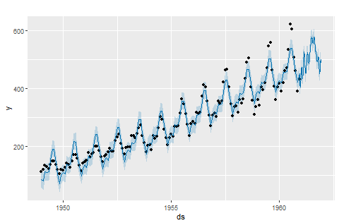
Output: Above graph shows the forecasted values of AirPassengers where, Black dots refers to the original data, Dark blue line refers to the predicted value(yhat), and Light blue area indicates the yhat_upper and yhat_lower value. Step 8: Plot the trend, weekly and yearly seasonality

# Output to be present
# As PNG file
png(file = "facebookprophettrendGFG.png")

# Plot
prophet_plot_components(m, forecast)

# Saving the file
dev.off()

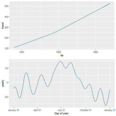
Output: The above graph shows the trend of the dataset that air passengers have been increased over a given period of time. In second graph, it shows seasonality of the dataset over a period of time i.e., yearly and signifies that air passengers were maximum between months from June to August.