RFM Analysis Analysis Using Python

In this article, we are going to see Recency, Frequency, Monetary value analysis using Python. But first, let us understand the RFM analysis briefly.

What is RFM analysis?

RFM stands for recency, frequency, monetary value. In business analytics, we often use this concept to divide customers into different segments, like high-value customers, medium value customers or low-value customers, and similarly many others.

Let’s assume we are a company, our company name is geek, let’s perform the RFM analysis on our customers

1. Recency: How recently has the customer made a transaction with us
2. Frequency: How frequent is the customer in ordering/buying some product from us
3. Monetary: How much does the customer spend on purchasing products from us.

Getting Started

Loading the necessary libraries and the data

Here we will import the required module( pandas, DateTime, and NumPy) and then read the data in the dataframe.

Dataset Used: rfm

Python3

# importing necessary libraries
import pandas as pd
import datetime as dt
import numpy as np

# importing the data
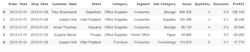
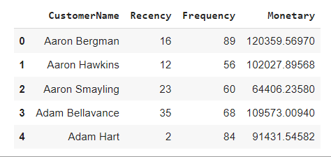
df = pd.read_excel( < my excel file location > )
df.head()

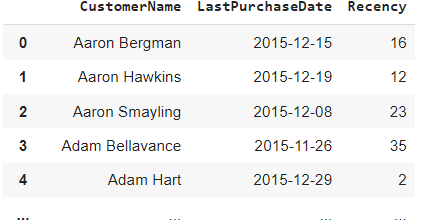
Calculating Recency

Here we are calculating recency for customers who had made a purchase with a company.

Python3

df_recency = df.groupby(by='Customer Name',
                        as_index=False)['Order Date'].max()
df_recency.columns = ['CustomerName', 'LastPurchaseDate']
recent_date = df_recency['LastPurchaseDate'].max()
df_recency['Recency'] = df_recency['LastPurchaseDate'].apply(
    lambda x: (recent_date - x).days)
df_recency.head()

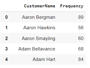
Calculating Frequency

We are here calculating the frequency of frequent transactions of the customer in ordering/buying some product from the company.

Python3

frequency_df = df.drop_duplicates().groupby(
    by=['Customer Name'], as_index=False)['Order Date'].count()
frequency_df.columns = ['CustomerName', 'Frequency']
frequency_df.head()

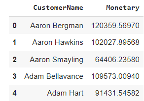
Calculating Monetary Value

Here we are calculating the monetary value of customer spend on purchasing products from the company.

Python3

df['Total'] = df['Sales']*df['Quantity']
monetary_df = df.groupby(by='Customer Name', as_index=False)['Total'].sum()
monetary_df.columns = ['CustomerName', 'Monetary']
monetary_df.head()

Merging all three columns in one dataframe

Here we are merging all the dataframe columns in a single entity using the merge function to display the recency, frequency, monetary value.

Python3

rf_df = df_recency.merge(frequency_df, on='CustomerName')
rfm_df = rf_df.merge(monetary_df, on='CustomerName').drop(
    columns='LastPurchaseDate')
rfm_df.head()

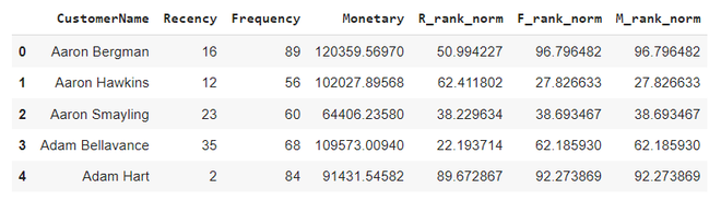
Ranking Customer’s based upon their recency, frequency, and monetary score

Here we are normalizing the rank of the customers within a company to analyze the ranking.

Python3

rfm_df['R_rank'] = rfm_df['Recency'].rank(ascending=False)
rfm_df['F_rank'] = rfm_df['Frequency'].rank(ascending=True)
rfm_df['M_rank'] = rfm_df['Monetary'].rank(ascending=True)

# normalizing the rank of the customers
rfm_df['R_rank_norm'] = (rfm_df['R_rank']/rfm_df['R_rank'].max())*100
rfm_df['F_rank_norm'] = (rfm_df['F_rank']/rfm_df['F_rank'].max())*100
rfm_df['M_rank_norm'] = (rfm_df['F_rank']/rfm_df['M_rank'].max())*100

rfm_df.drop(columns=['R_rank', 'F_rank', 'M_rank'], inplace=True)

rfm_df.head()

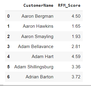
Calculating RFM score

RFM score is calculated based upon recency, frequency, monetary value normalize ranks. Based upon this score we divide our customers. Here we rate them on a scale of 5. Formula used for calculating rfm score is : 0.15*Recency score + 0.28*Frequency score + 0.57 *Monetary score

Python3

rfm_df['RFM_Score'] = 0.15*rfm_df['R_rank_norm']+0.28 * \
    rfm_df['F_rank_norm']+0.57*rfm_df['M_rank_norm']
rfm_df['RFM_Score'] *= 0.05
rfm_df = rfm_df.round(2)
rfm_df[['CustomerName', 'RFM_Score']].head(7)

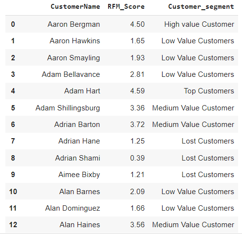
Rating Customer based upon the RFM score

• rfm score >4.5 : Top Customer
• 4.5 > rfm score > 4 : High Value Customer
• 4>rfm score >3 : Medium value customer
• 3>rfm score>1.6 : Low-value customer
• rfm score<1.6 :Lost Customer

Python3

rfm_df["Customer_segment"] = np.where(rfm_df['RFM_Score'] >
                                      4.5, "Top Customers",
                                      (np.where(
                                        rfm_df['RFM_Score'] > 4,
                                        "High value Customer",
                                        (np.where(
    rfm_df['RFM_Score'] > 3,
                             "Medium Value Customer",
                             np.where(rfm_df['RFM_Score'] > 1.6,
                            'Low Value Customers', 'Lost Customers'))))))
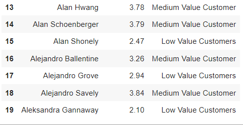
rfm_df[['CustomerName', 'RFM_Score', 'Customer_segment']].head(20)

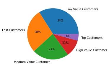
Visualizing the customer segments

Here we will use a pie plot to display all segments of customers.

Python3

plt.pie(rfm_df.Customer_segment.value_counts(),
        labels=rfm_df.Customer_segment.value_counts().index,
        autopct='%.0f%%')
plt.show()