Time Series Analysis using Facebook Prophet

Time series analysis is one of the important methodologies that helps us to understand the hidden patterns in a dataset that is too related to the time at which it is being recorded. The article aims to explore the fundamentals of time series analysis and demonstrates the analysis using Facebook Prophet.

What is Time Series Analysis?

Time series analysis is a statistical approach that entails gathering data at consistent intervals to recognize patterns and trends. This methodology is employed for making well-informed decisions and precise forecasts by leveraging insights derived from historical data.

And the process of predicting the future values of the data by analyzing the previous trends and patterns hidden in the data is known as time series forecasting. Time series forecasting can be done using various forecasting techniques like ARIMA, SARIMA, Prophet, Theta and other statistical method. Time series data is a sequential data hence, deep learning-based methods like RNN, LSTM, BLSTM and GRU are also used for time series forecasting.

Key components of Time Series analysis

The key components of time series analysis include:

1. Time series data commonly displays temporal relationships, meaning that the values at a particular moment are impacted by preceding values. Grasping these dependencies is essential for accurate predictions and gaining valuable insights.
2. Trend analysis involves recognizing the fundamental direction or long-term movement in a time series, whether it is upward, downward, or stable. This understanding provides insights into the overall trajectory of the data.
3. Seasonal patterns, observed in numerous time series, depict recurring cycles at fixed intervals, such as daily, monthly, quarterly, or yearly. Analyzing these patterns through seasonal analysis helps identify and comprehend their periodic nature.
4. Time series data often incorporates random fluctuations or noise that lacks a specific trend or pattern. It is crucial to eliminate this noise to unveil meaningful information within the data.

Facebook Prophet Library

Prophet is an open-source tool from Facebook used for forecasting time series data which helps businesses understand and possibly predict the market. It is based on a decomposable additive model where non-linear trends fit with seasonality, it also takes into account the effects of holidays. Before we head right into coding, let’s learn certain terms that are required to understand this. 

• Trend: The trend shows the tendency of the data to increase or decrease over a long period of time and it filters out the seasonal variations. 
• Seasonality: Seasonality is the variations that occur over a short period of time and is not prominent enough to be called a “trend”. 

Understanding the Prophet Model

The general idea of the model is similar to a generalized additive model. The “Prophet Equation” fits, as mentioned above, trends, seasonality, and holidays. This is given by,

y(t) = g(t) + s(t) + h(t) + e(t)

here,

• g(t) refers to trend (changes over a long period of time)
• s(t) refers to seasonality (periodic or short-term changes)
• h(t) refers to effects of holidays to the forecast
• e(t) refers to the unconditional changes that is specific to a business or a person or a circumstance. It is also called the error term.
• y(t) is the forecast.

Need of Facebook Prophet

We need it because, although the basic decomposable additive model looks simply, the calculation of the terms within is hugely mathematical. If you do not know what you are doing, it may lead to making wrong forecasts, which might have severe repercussions in the real world. So, to automate this process, we are going to use Prophet. However, to understand the math behind this process and how Prophet actually works, let’s see how it forecasts the data. 

Prophet provides us with two models (however, newer models can be written or extended according to specific requirements). 

1. Logistic Growth Model 
2. Piece-Wise Linear Model

By default, Prophet uses a piece-wise linear model, but it can be changed by specifying the model. Choosing a model is delicate as it is dependent on a variety of factors such as company size, growth rate, business model, etc., If the data to be forecasted, has saturating and non-linear data (grows non-linearly and after reaching the saturation point, shows little to no growth or shrink and only exhibits some seasonal changes), then logistic growth model is the best option. Nevertheless, if the data shows linear properties and had growth or shrink trends in the past then, the piece-wise linear model is a better choice. The logistic growth model is fit using the following statistical equation, 

where,

• C is the carrying capacity
• k is the growth rate
• m is an offset parameter

The piece-wise linear model is fit using the following statistical equations,  

(1)

where c is the trend change point (it defines the change in the trend).? is the trend parameter and can be tuned as per requirement for forecasting.  

Implementation – Analyzing Time Series Data using Prophet

Now let’s try and build a model that is going to forecast the number of passengers for the next five years using time series analysis.

Installing Prophet and Other Dependencies

Install pandas for data manipulation and for the dataframe data structure.

!pip install pandas

Install Prophet for time series analysis and forecasting.

!pip install prophet

Importing Required Libraries

Python3

import pandas as pd
from prophet import Prophet
from prophet.plot import add_changepoints_to_plot

Loading Air Passenger Dataset

Now let’s load the csv file in the pandas data frame. The dataset contains the number of air passengers in the USA from January 1949 to December 1960. The frequency of the data is 1 month.

Python3

url = ("https://raw.githubusercontent.com/rahulhegde99"
      "/Time-Series-Analysis-and-Forecasting-of-Air-Passengers"
        "/master/airpassengers.csv")
data = pd.read_csv(url)
data.head()

Output:

     Month  #Passengers
0  1949-01          112
1  1949-02          118
2  1949-03          132
3  1949-04          129
4  1949-05          121

Facebook Prophet predicts data only when it is in a certain format. The dataframe with the data should have a column saved as ds for time series data and y for the data to be forecasted. Here, the time series is the column Month and the data to be forecasted is the column #Passengers. So, let’s make a new DataFrame with new column names and the same data. Also, ds should be in a DateTime format.

Python3

df = pd.DataFrame()
df['ds'] = pd.to_datetime(data['Month'])
df['y'] = data['#Passengers']
df.head()

Output:

          ds    y
0 1949-01-01  112
1 1949-02-01  118
2 1949-03-01  132
3 1949-04-01  129
4 1949-05-01  121

Initializing a Prophet Model

By using the Prophet() command we can initialize an instance of the fbprophet model for the training on our dataset and then help us to perform time series forecasting.

Python3

m = Prophet()
m.fit(df)

We want our model to predict the next 5 years, that is, till 1965. The frequency of our data is 1 month and thus for 5 years, it is 12 * 5 = 60 months. So, we need to add 60 to more rows of monthly data to a dataframe.

Python3

future = m.make_future_dataframe(periods=12 * 5,
                                 freq='M')

Now in the future dataframe we have just ds values, and we should predict the y values.

Python3

forecast = m.predict(future)
forecast[['ds', 'yhat', 'yhat_lower',
          'yhat_upper', 'trend',
          'trend_lower', 'trend_upper']].tail()

Output:

            ds        yhat  yhat_lower  yhat_upper       trend  trend_lower  \
199 1965-07-31  723.847886  695.131427  753.432671  656.874802   649.871409   
200 1965-08-31  677.972773  649.074148  707.203918  660.006451   652.869703   
201 1965-09-30  640.723643  612.025440  670.377970  663.037079   655.722042   
202 1965-10-31  610.965273  580.772823  641.770085  666.168728   658.710202   
203 1965-11-30  640.594175  611.016447  669.582208  669.199356   661.513728   

     trend_upper  
199   663.255178  
200   666.675498  
201   669.917580  
202   673.241446  
203   676.479915  

Plotting the Forecast Data

Table ds, as we know, is the time series data. yhat is the prediction, yhat_lower, and yhat_upper are the uncertainty levels (it basically means the prediction and actual values can vary within the bounds of the uncertainty levels). Next up we have a trend that shows the long-term growth, shrink, or stagnancy of the data, trend_lower, and trend_upper is the uncertainty levels.

Python3

fig1 = m.plot(forecast, include_legend=True)

Output:

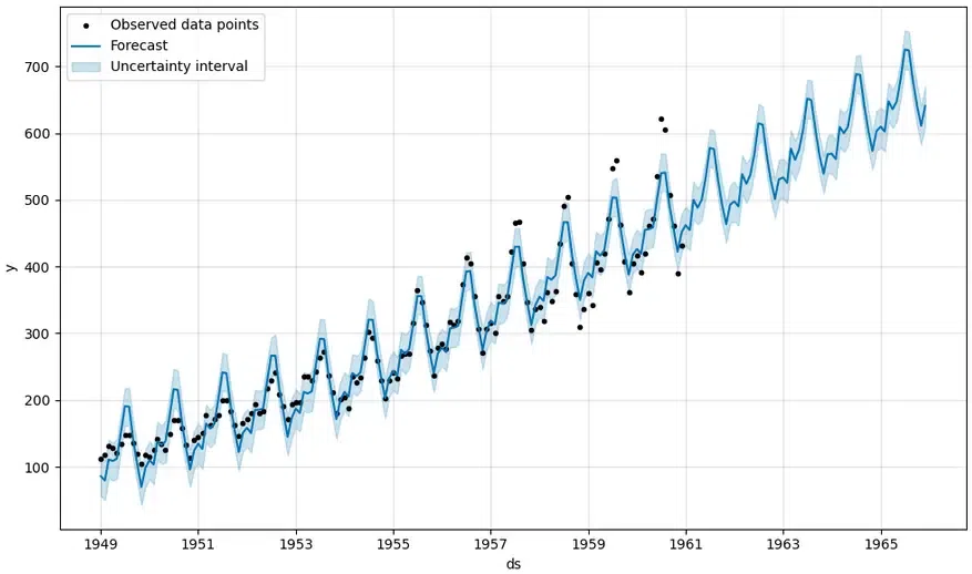
Time Series Forecasting

The below image shows the basic prediction. The light blue is the uncertainty level(yhat_upper and yhat_lower), the dark blue is the prediction(yhat) and the black dots are the original data. We can see that the predicted data is very close to the actual data. In the last five years, there is no “actual” data, but looking at the performance of our model in years where data is available it is safe to say that the predictions are close to accurate.

Python3

fig2 = m.plot_components(forecast)

Output:

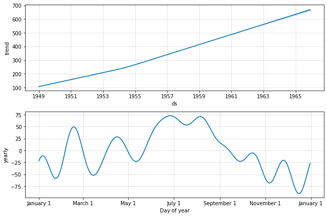
Trends and Seasonality in Time Series Data

The below images show the trends and seasonality (in a year) of the time series data. We can see there is an increasing trend, meaning the number of air passengers has increased over time. If we look at the seasonality graph, we can see that June and July is the time with the most passengers in a given year.

Python3

fig = m.plot(forecast)
a = add_changepoints_to_plot(fig.gca(),
                             m, forecast)

Output:

Forecasting using Prophet

Add changepoints to indicate the time in rapid trend growths. The dotted red lines show the time when there was a rapid change in the trend of the passengers. Thus, we have seen how we can design a prediction model using Facebook Prophet with only a few lines of code which would have been very difficult to implement using traditional machine learning algorithms and mathematical and statistical concepts alone.