Time Series Analysis and Forecasting

Time series analysis and forecasting are crucial for predicting future trends, behaviors, and behaviours based on historical data. It helps businesses make informed decisions, optimize resources, and mitigate risks by anticipating market demand, sales fluctuations, stock prices, and more. Additionally, it aids in planning, budgeting, and strategizing across various domains such as finance, economics, healthcare, climate science, and resource management, driving efficiency and competitiveness.

What is a Time Series?

A time series is a sequence of data points collected, recorded, or measured at successive, evenly-spaced time intervals.

Each data point represents observations or measurements taken over time, such as stock prices, temperature readings, or sales figures. Time series data is commonly represented graphically with time on the horizontal axis and the variable of interest on the vertical axis, allowing analysts to identify trends, patterns, and changes over time.

Time series data is often represented graphically as a line plot, with time depicted on the horizontal x-axis and the variable’s values displayed on the vertical y-axis. This graphical representation facilitates the visualization of trends, patterns, and fluctuations in the variable over time, aiding in the analysis and interpretation of the data.

Importance of Time Series Analysis

1. Predict Future Trends: Time series analysis enables the prediction of future trends, allowing businesses to anticipate market demand, stock prices, and other key variables, facilitating proactive decision-making.
2. Detect Patterns and Anomalies: By examining sequential data points, time series analysis helps detect recurring patterns and anomalies, providing insights into underlying behaviors and potential outliers.
3. Risk Mitigation: By spotting potential risks, businesses can develop strategies to mitigate them, enhancing overall risk management.
4. Strategic Planning: Time series insights inform long-term strategic planning, guiding decision-making across finance, healthcare, and other sectors.
5. Competitive Edge: Time series analysis enables businesses to optimize resource allocation effectively, whether it’s inventory, workforce, or financial assets. By staying ahead of market trends, responding to changes, and making data-driven decisions, businesses gain a competitive edge.

Components of Time Series Data

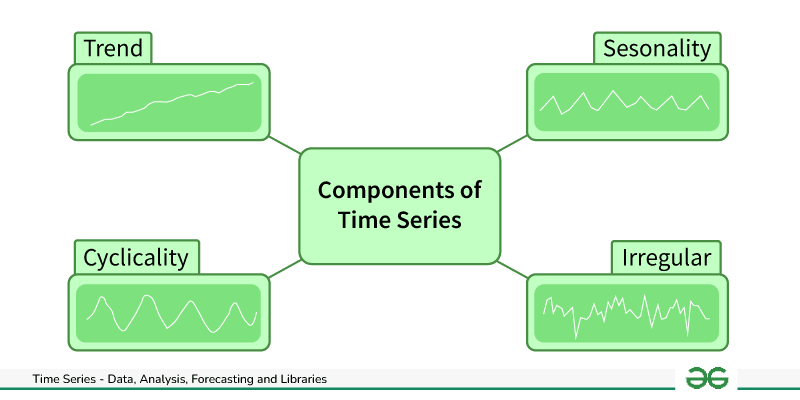
There are four main components of a time series:

Components of Time Series Data

1. Trend: Trend represents the long-term movement or directionality of the data over time. It captures the overall tendency of the series to increase, decrease, or remain stable. Trends can be linear, indicating a consistent increase or decrease, or nonlinear, showing more complex patterns.
2. Seasonality: Seasonality refers to periodic fluctuations or patterns that occur at regular intervals within the time series. These cycles often repeat annually, quarterly, monthly, or weekly and are typically influenced by factors such as seasons, holidays, or business cycles.
3. Cyclic variations: Cyclical variations are longer-term fluctuations in the time series that do not have a fixed period like seasonality. These fluctuations represent economic or business cycles, which can extend over multiple years and are often associated with expansions and contractions in economic activity.
4. Irregularity (or Noise): Irregularity, also known as noise or randomness, refers to the unpredictable or random fluctuations in the data that cannot be attributed to the trend, seasonality, or cyclical variations. These fluctuations may result from random events, measurement errors, or other unforeseen factors. Irregularity makes it challenging to identify and model the underlying patterns in the time series data.

Time Series Visualization

Time series visualization is the graphical representation of data collected over successive time intervals. It encompasses various techniques such as line plots, seasonal subseries plots, autocorrelation plots, histograms, and interactive visualizations. These methods help analysts identify trends, patterns, and anomalies in time-dependent data for better understanding and decision-making.

Different Time series visualization graphs

1. Line Plots: Line plots display data points over time, allowing easy observation of trends, cycles, and fluctuations.
2. Seasonal Plots: These plots break down time series data into seasonal components, helping to visualize patterns within specific time periods.
3. Histograms and Density Plots: Shows the distribution of data values over time, providing insights into data characteristics such as skewness and kurtosis.
4. Autocorrelation and Partial Autocorrelation Plots: These plots visualize correlation between a time series and its lagged values, helping to identify seasonality and lagged relationships.
5. Spectral Analysis: Spectral analysis techniques, such as periodograms and spectrograms, visualize frequency components within time series data, useful for identifying periodicity and cyclical patterns.
6. Decomposition Plots: Decomposition plots break down a time series into its trend, seasonal, and residual components, aiding in understanding the underlying patterns.

These visualization techniques allow analysts to explore, interpret, and communicate insights from time series data effectively, supporting informed decision-making and forecasting.

Time Series Visualization Techniques: Python and R Implementations

Time series Visualization	Python implementations	R Implementations
Line Plots	Read here	Read here
Seasonal Plots	Read here	Read here
Histograms and Density Plots over time	Read here	Read here
Decomposition Plots	Read here	Read here
Spectral Analysis	Read here	Read here

Preprocessing Time Series Data

Time series preprocessing refers to the steps taken to clean, transform, and prepare time series data for analysis or forecasting. It involves techniques aimed at improving data quality, removing noise, handling missing values, and making the data suitable for modeling. Preprocessing tasks may include removing outliers, handling missing values through imputation, scaling or normalizing the data, detrending, deseasonalizing, and applying transformations to stabilize variance. The goal is to ensure that the time series data is in a suitable format for subsequent analysis or modeling.

• Handling Missing Values : Dealing with missing values in the time series data to ensure continuity and reliability in analysis.
• Dealing with Outliers: Identifying and addressing observations that significantly deviate from the rest of the data, which can distort analysis results.
• Stationarity and Transformation: Ensuring that the statistical properties of the time series, such as mean and variance, remain constant over time. Techniques like differencing, detrending, and deseasonalizing are used to achieve stationarity.

Time Series Preprocessing Techniques: Python and R Implementations

Time Series Preprocessing Techniques	Python implementations	R Implementations
Stationarity	Read here	Read here
Differencing	Read here	Read here
Detrending	Read here	Read here
Deseasonalizing	Read here	Read here
Moving Average	Read here	Read here
Exponential Moving Average	Read here	Read here
Missing Value Imputation	Read here	Read here
Outlier Detection and Removal	Read here	Read here
Time Alignment	Read here	Read here
Data Transformation	Read here	Read here
Scaling	Read here	Read here
Normalization	Read here	Read here

Time Series Analysis & Decomposition

Time Series Analysis and Decomposition is a systematic approach to studying sequential data collected over successive time intervals. It involves analyzing the data to understand its underlying patterns, trends, and seasonal variations, as well as decomposing the time series into its fundamental components. This decomposition typically includes identifying and isolating elements such as trend, seasonality, and residual (error) components within the data.

Different Time Series Analysis & Decomposition Techniques

1. Autocorrelation Analysis: A statistical method to measure the correlation between a time series and a lagged version of itself at different time lags. It helps identify patterns and dependencies within the time series data.
2. Partial Autocorrelation Functions (PACF): PACF measures the correlation between a time series and its lagged values, controlling for intermediate lags, aiding in identifying direct relationships between variables.
3. Trend Analysis: The process of identifying and analyzing the long-term movement or directionality of a time series. Trends can be linear, exponential, or nonlinear and are crucial for understanding underlying patterns and making forecasts.
4. Seasonality Analysis: Seasonality refers to periodic fluctuations or patterns that occur in a time series at fixed intervals, such as daily, weekly, or yearly. Seasonality analysis involves identifying and quantifying these recurring patterns to understand their impact on the data.
5. Decomposition: Decomposition separates a time series into its constituent components, typically trend, seasonality, and residual (error). This technique helps isolate and analyze each component individually, making it easier to understand and model the underlying patterns.
6. Spectrum Analysis: Spectrum analysis involves examining the frequency domain representation of a time series to identify dominant frequencies or periodicities. It helps detect cyclic patterns and understand the underlying periodic behavior of the data.
7. Seasonal and Trend decomposition using Loess: STL decomposes a time series into three components: seasonal, trend, and residual. This decomposition enables modeling and forecasting each component separately, simplifying the forecasting process.
8. Rolling Correlation: Rolling correlation calculates the correlation coefficient between two time series over a rolling window of observations, capturing changes in the relationship between variables over time.
9. Cross-correlation Analysis: Cross-correlation analysis measures the similarity between two time series by computing their correlation at different time lags. It is used to identify relationships and dependencies between different variables or time series.
10. Box-Jenkins Method: Box-Jenkins Method is a systematic approach for analyzing and modeling time series data. It involves identifying the appropriate autoregressive integrated moving average (ARIMA) model parameters, estimating the model, diagnosing its adequacy through residual analysis, and selecting the best-fitting model.
11. Granger Causality Analysis: Granger causality analysis determines whether one time series can predict future values of another time series. It helps infer causal relationships between variables in time series data, providing insights into the direction of influence.

Time Series Analysis & Decomposition Techniques: Python and R Implementations

Time Series Analysis Techniques	Python implementations	R implementations
Autocorrelation Analysis	Read here	Read here
Partial Autocorrelation Functions (PACF)	Read here	Read here
Trend Analysis	Read here	Read here
Seasonality Analysis	Read here	Read here
Decomposition	Read here	Read here
Spectrum Analysis	Read here	Read here
Seasonal and Trend decomposition using Loess (STL)	Read here	Read here
Rolling correlation	Read here	Read here
Cross-correlation Analysis	Read here	Read here
Box-Jenkins Method	Read here	Read here
Granger Causality Analysis	Read here	Read here

What is Time Series Forecasting?

Time Series Forecasting is a statistical technique used to predict future values of a time series based on past observations. In simpler terms, it’s like looking into the future of data points plotted over time. By analyzing patterns and trends in historical data, Time Series Forecasting helps make informed predictions about what may happen next, assisting in decision-making and planning for the future.

Different Time Series Forecasting Algorithms

1. Autoregressive (AR) Model: Autoregressive (AR) model is a type of time series model that predicts future values based on linear combinations of past values of the same time series. In an AR(p) model, the current value of the time series is modeled as a linear function of its previous p values, plus a random error term. The order of the autoregressive model (p) determines how many past values are used in the prediction.
2. Autoregressive Integrated Moving Average (ARIMA): ARIMA is a widely used statistical method for time series forecasting. It models the next value in a time series based on linear combination of its own past values and past forecast errors. The model parameters include the order of autoregression (p), differencing (d), and moving average (q).
3. ARIMAX: ARIMA model extended to include exogenous variables that can improve forecast accuracy.
4. Seasonal Autoregressive Integrated Moving Average (SARIMA): SARIMA extends ARIMA by incorporating seasonality into the model. It includes additional seasonal parameters (P, D, Q) to capture periodic fluctuations in the data.
5. SARIMAX: Extension of SARIMA that incorporates exogenous variables for seasonal time series forecasting.
6. Vector Autoregression (VAR) Models: VAR models extend autoregression to multivariate time series data by modeling each variable as a linear combination of its past values and the past values of other variables. They are suitable for analyzing and forecasting interdependencies among multiple time series.
7. Theta Method: A simple and intuitive forecasting technique based on extrapolation and trend fitting.
8. Exponential Smoothing Methods: Exponential smoothing methods, such as Simple Exponential Smoothing (SES) and Holt-Winters, forecast future values by exponentially decreasing weights for past observations. These methods are particularly useful for data with trend and seasonality.
9. Gaussian Processes Regression: Gaussian Processes Regression is a Bayesian non-parametric approach that models the distribution of functions over time. It provides uncertainty estimates along with point forecasts, making it useful for capturing uncertainty in time series forecasting.
10. Generalized Additive Models (GAM): A flexible modeling approach that combines additive components, allowing for nonlinear relationships and interactions.
11. Random Forests: Random Forests is a machine learning ensemble method that constructs multiple decision trees during training and outputs the average prediction of the individual trees. It can handle complex relationships and interactions in the data, making it effective for time series forecasting.
12. Gradient Boosting Machines (GBM): GBM is another ensemble learning technique that builds multiple decision trees sequentially, where each tree corrects the errors of the previous one. It excels in capturing nonlinear relationships and is robust against overfitting.
13. State Space Models: State space models represent a time series as a combination of unobserved (hidden) states and observed measurements. These models capture both the deterministic and stochastic components of the time series, making them suitable for forecasting and anomaly detection.
14. Dynamic Linear Models (DLMs): DLMs are Bayesian state-space models that represent time series data as a combination of latent state variables and observations. They are flexible models capable of incorporating various trends, seasonality, and other dynamic patterns in the data.
15. Recurrent Neural Networks (RNNs) and Long Short-Term Memory (LSTM) Networks: RNNs and LSTMs are deep learning architectures designed to handle sequential data. They can capture complex temporal dependencies in time series data, making them powerful tools for forecasting tasks, especially when dealing with large-scale and high-dimensional data.
16. Hidden Markov Model (HMM): A Hidden Markov Model (HMM) is a statistical model used to describe sequences of observable events generated by underlying hidden states. In time series, HMMs infer hidden states from observed data, capturing dependencies and transitions between states. They are valuable for tasks like speech recognition, gesture analysis, and anomaly detection, providing a framework to model complex sequential data and extract meaningful patterns from it.

Time Series Forecasting Algorithms: Python and R Implementations

Time Series Forecasting Algorithms	Python implementations	R implementations
Autoregressive (AR) Model	Read here	Read here
ARIMA	Read here	Read here
ARIMAX	Read here	Read here
SARIMA	Read here	Read here
SARIMAX	Read here	Read here
Vector Autoregression (VAR)	Read here	Read here
Theta Method	Read here	Read here
Exponential Smoothing Methods	Read here	Read here
Gaussian Processes Regression	Read here	Read here
Generalized Additive Models (GAM)	Read here	Read here
Random Forests	Read here	Read here
Gradient Boosting Machines (GBM)	Read here	Read here
State Space Models	Read here	Read here
Hidden Markov Model (HMM)	Read here	Read here
Dynamic Linear Models (DLMs)	Read here	Read here
Recurrent Neural Networks (RNNs)	Read here	Read here
Long Short-Term Memory (LSTM)	Read here	Read here
Gated Recurrent Unit (GRU)	Read here	Read here

Evaluating Time Series Forecasts

Evaluating Time Series Forecasts involves assessing the accuracy and effectiveness of predictions made by time series forecasting models. This process aims to measure how well a model performs in predicting future values based on historical data. By evaluating forecasts, analysts can determine the reliability of the models, identify areas for improvement, and make informed decisions about their use in practical applications.

Performance Metrics:

Performance metrics are quantitative measures used to evaluate the accuracy and effectiveness of time series forecasts. These metrics provide insights into how well a forecasting model performs in predicting future values based on historical data. Common performance metrics which can be used for time series include:

1. Mean Absolute Error (MAE): Measures the average magnitude of errors between predicted and actual values.
2. Mean Absolute Percentage Error (MAPE): Calculates the average percentage difference between predicted and actual values.
3. Mean Squared Error (MSE): Computes the average squared differences between predicted and actual values.
4. Root Mean Squared Error (RMSE): The square root of MSE, providing a measure of the typical magnitude of errors.
5. Forecast Bias: Determines whether forecasts systematically overestimate or underestimate actual values.
6. Forecast Interval Coverage: Evaluates the percentage of actual values that fall within forecast intervals.
7. Theil’s U Statistic: Compares the performance of the forecast model to a naïve benchmark model.

Cross-Validation Techniques

Cross-validation techniques are used to assess the generalization performance of time series forecasting models. These techniques involve splitting the available data into training and testing sets, fitting the model on the training data, and evaluating its performance on the unseen testing data. Common cross-validation techniques for time series data include:

1. Train-Test Split for Time Series: Divides the dataset into a training set for model fitting and a separate testing set for evaluation.
2. Rolling Window Validation: Uses a moving window approach to iteratively train and test the model on different subsets of the data.
3. Time Series Cross-Validation: Splits the time series data into multiple folds, ensuring that each fold maintains the temporal order of observations.
4. Walk-Forward Validation: Similar to rolling window validation but updates the training set with each new observation, allowing the model to adapt to changing data patterns.

Top Python Libraries for Time Series Analysis & Forecasting

Python Libraries for Time Series Analysis & Forecasting encompass a suite of powerful tools and frameworks designed to facilitate the analysis and forecasting of time series data. These libraries offer a diverse range of capabilities, including statistical modeling, machine learning algorithms, deep learning techniques, and probabilistic forecasting methods. With their user-friendly interfaces and extensive documentation, these libraries serve as invaluable resources for both beginners and experienced practitioners in the field of time series analysis and forecasting.

1. Statsmodels: Statsmodels is a Python library for statistical modeling and hypothesis testing. It includes a wide range of statistical methods and models, including time series analysis tools like ARIMA, SARIMA, and VAR. Statsmodels is useful for performing classical statistical tests and building traditional time series models.
2. Pmdarima: Pmdarima is a Python library that provides an interface to ARIMA models in a manner similar to that of scikit-learn. It automates the process of selecting optimal ARIMA parameters and fitting models to time series data.
3. Prophet: Prophet is a forecasting tool developed by Facebook that is specifically designed for time series forecasting at scale. It provides a simple yet powerful interface for fitting and forecasting time series data, with built-in support for handling seasonality, holidays, and trend changes.
4. tslearn: tslearn is a Python library for time series learning, which provides various algorithms and tools for time series classification, clustering, and regression. It offers implementations of state-of-the-art algorithms, such as dynamic time warping (DTW) and shapelets, for analyzing and mining time series data.
5. ARCH: ARCH is a Python library for estimating and forecasting volatility models commonly used in financial econometrics. It provides tools for fitting autoregressive conditional heteroskedasticity (ARCH) and generalized autoregressive conditional heteroskedasticity (GARCH) models to time series data.
6. GluonTS: GluonTS is a Python library for probabilistic time series forecasting developed by Amazon. It provides a collection of state-of-the-art deep learning models and tools for building and training probabilistic forecasting models for time series data.
7. PyFlux: PyFlux is a Python library for time series analysis and forecasting, which provides implementations of various time series models, including ARIMA, GARCH, and stochastic volatility models. It offers an intuitive interface for fitting and forecasting time series data with Bayesian inference methods.
8. Sktime: Sktime is a Python library for machine learning with time series data, which provides a unified interface for building and evaluating machine learning models for time series forecasting, classification, and regression tasks. It integrates seamlessly with scikit-learn and offers tools for handling time series data efficiently.
9. PyCaret: PyCaret is an open-source, low-code machine learning library in Python that automates the machine learning workflow. It supports time series forecasting tasks and provides tools for data preprocessing, feature engineering, model selection, and evaluation in a simple and streamlined manner.
10. Darts: Darts (Data Augmentation for Regression Tasks with SVD) is a Python library for time series forecasting. It provides a flexible and modular framework for developing and evaluating forecasting models, including classical and deep learning-based approaches. Darts emphasizes simplicity, scalability, and reproducibility in time series analysis and forecasting tasks.
11. Kats: Kats, short for “Kits to Analyze Time Series,” is an open-source Python library developed by Facebook. It provides a comprehensive toolkit for time series analysis, offering a wide range of functionalities to handle various aspects of time series data. Kats includes tools for time series forecasting, anomaly detection, feature engineering, and model evaluation. It aims to simplify the process of working with time series data by providing an intuitive interface and a collection of state-of-the-art algorithms.
12. AutoTS: AutoTS, or Automated Time Series, is a Python library developed to simplify time series forecasting by automating the model selection and parameter tuning process. It employs machine learning algorithms and statistical techniques to automatically identify the most suitable forecasting models and parameters for a given dataset. This automation saves time and effort by eliminating the need for manual model selection and tuning.
13. Scikit-learn: Scikit-learn is a popular machine learning library in Python that provides a wide range of algorithms and tools for data mining and analysis. While not specifically tailored for time series analysis, Scikit-learn offers some useful algorithms for forecasting tasks, such as regression, classification, and clustering.
14. TensorFlow: TensorFlow is an open-source machine learning framework developed by Google. It is widely used for building and training deep learning models, including recurrent neural networks (RNNs) and long short-term memory networks (LSTMs), which are commonly used for time series forecasting tasks.
15. Keras: Keras is a high-level neural networks API written in Python, which runs on top of TensorFlow. It provides a user-friendly interface for building and training neural networks, including recurrent and convolutional neural networks, for various machine learning tasks, including time series forecasting.
16. PyTorch: PyTorch is another popular deep learning framework that is widely used for building neural network models. It offers dynamic computation graphs and a flexible architecture, making it suitable for prototyping and experimenting with complex models for time series forecasting.

Comparative Analysis of Python Libraries for Time Series

Python offers a diverse range of libraries and frameworks tailored for time series tasks, each with its own set of strengths and weaknesses. In this comparative analysis, we evaluate top Python libraries, which is commonly used for time series analysis and forecasting.

Framework or Libraries	Focus Area	Strengths	Weaknesses
Statsmodels	Statistics	Extensive support for classical time series models like ARIMA and SARIMA.	Limited machine learning capabilities.
Pmdarima	ARIMA Forecasting	Simplifies ARIMA model selection and tuning.	Limited to ARIMA-based forecasting; lacks broader statistical modeling capabilities.
Prophet	Business Forecasting	User-friendly for forecasting with seasonality, holidays, and explanatory variables.	Limited flexibility for customization; less suitable for complex time series with irregular patterns.
tslearn	Machine Learning	Specialized machine learning algorithms for time series tasks like classification and clustering.	Limited support for classical statistical modeling; may require additional libraries for certain analyses.
ARCH	Financial Econometrics	Specifically designed for modeling financial time series with ARCH/GARCH models.	Focuses primarily on financial time series; may not be suitable for general-purpose time series analysis.
GluonTS	Deep Learning	Deep learning framework for time series forecasting with built-in models.	Requires familiarity with deep learning concepts and MXNet framework.
PyFlux	Deep Learning	Deep learning framework for time series forecasting, built on PyTorch.	Requires familiarity with deep learning concepts and PyTorch framework.
Sktime	Machine Learning	Unifying framework for various machine learning tasks on time series data.	Still under development; may lack maturity compared to established libraries.
PyCaret	AutoML	Automated machine learning for time series forecasting, simplifies model selection.	Limited control over individual models; less suitable for advanced users requiring customizations.
Darts	Probabilistic Forecasting	Probabilistic forecasting models; offers uncertainty quantification.	Steeper learning curve compared to simpler libraries; may require advanced statistical knowledge.
Kats	Bayesian Forecasting	Bayesian approach to time series forecasting. Good for handling missing data.	Less user-friendly interface compared to some options. Relatively new library.
AutoTS	Automated Forecasting	Automatic time series forecasting with hyperparameter tuning.	Limited control over specific models used. Less transparency in the forecasting process.
Scikit-learn	Machine Learning	Offers basic time series functionalities through specific transformers and estimators.	Not specifically designed for time series analysis. Limited forecasting capabilities.
TensorFlow	Deep Learning	Powerful deep learning framework, can be used for time series forecasting with custom models.	Requires significant coding expertise and deep learning knowledge.
Keras	Deep Learning API	High-level API for building deep learning models, can be used for time series forecasting.	Requires knowledge of deep learning concepts and underlying framework.
PyTorch	Deep Learning	Popular deep learning framework, can be used for time series forecasting with custom models.	Requires significant coding expertise and deep learning knowledge.

This table provides an overview of each library’s focus area, strengths, and weaknesses in the context of time series analysis and forecasting.

Conclusion

Python offers a rich ecosystem of libraries and frameworks tailored for time series analysis and forecasting, catering to diverse needs across various domains. From traditional statistical modeling with libraries like Statsmodels to cutting-edge deep learning approaches enabled by TensorFlow and PyTorch, practitioners have a wide array of tools at their disposal. However, each library comes with its own trade-offs in terms of usability, flexibility, and computational requirements. Choosing the right tool depends on the specific requirements of the task at hand, balancing factors like model complexity, interpretability, and computational efficiency. Overall, Python’s versatility and the breadth of available libraries empower analysts and data scientists to extract meaningful insights and make accurate predictions from time series data across different domains.

Frequently Asked Questions on Time Series Analysis

Q. What is time series data?

Time series data is a sequence of data points collected, recorded, or measured at successive, evenly spaced time intervals. It represents observations or measurements taken over time, such as stock prices, temperature readings, or sales figures.

Q. What are the four main components of a time series?

The four main components of a time series are:

1. Trend
2. Seasonality
3. Cyclical variations
4. Irregularity (or Noise)

Q. What is stationarity in time series?

Stationarity in time series refers to the property where the statistical properties of the data, such as mean and variance, remain constant over time. It indicates that the time series data does not exhibit trends or seasonality and is crucial for building accurate forecasting models.

Q. What is the real-time application of time series analysis and forecasting?

Time series analysis and forecasting have various real-time applications across different domains, including:

• Financial markets for predicting stock prices and market trends.
• Weather forecasting for predicting temperature, precipitation, and other meteorological variables.
• Energy demand forecasting for optimizing energy production and distribution.
• Healthcare for predicting patient admissions, disease outbreaks, and medical resource allocation.
• Retail for forecasting sales, demand, and inventory management.

Q. What do you mean by Dynamic Time Warping?

Dynamic Time Warping (DTW) is a technique used to measure the similarity between two sequences of data that may vary in time or speed. It aligns the sequences by stretching or compressing them in time to find the optimal matching between corresponding points. DTW is commonly used in time series analysis, speech recognition, and pattern recognition tasks where the sequences being compared have different lengths or rates of change.