Anomaly Detection in Time Series in R

Anomaly Detection in Time Series refers to finding data points or values that should not appear usually and have very unusual values. It plays a very important role in finding spikes or lows in a dataset and finding potential points of failure of any application due to it. Surges in internet traffic, DDoS attacks, etc. are monitored through anomaly detection. In this tutorial, we will learn to detect anomalies in the R Programming Language over a time series dataset.

Anomaly Detection in Time Series

Anomaly detection refers to the task of finding upper and lower thresholds of your dataset and then checking every row of the dataset whether it is an anomaly or not. To get the threshold, we need to find the trends of seasonality and residue.

• The trend is the long-term change over the dataset, where we can find the direction in which the data points are moving, be it upward, downward, or straight.
• Seasonality on the other hand is repeating patterns that occur. For example, before summer and winter vacations, there will be an increase in sales of holiday packages since schools and colleges shut down during that period.
• Finally, we find the residue that does not fit the trends and seasonality and can be considered an outlier.

Hence we can summarize the anomaly detection in the following steps

1. Exploring and finding the trends, seasonality and residue.
2. Finding the thresholds
3. Identifying the outliers

Monthly Electricity Consumption

In this example, we are going to explore the monthly electricity usage of a home and find the anomalies.

Dataset: Monthly Electricity Consumption Data

We are going to use the following two libraries:

• tidyverse: It makes it easy to install and load core packages from the tidyverse in a single command.
• anomalize: It provides a tidy workflow to find anomalies in the dataset.

Step 1: Load the libraries

R

library(tidyverse)
library(anomalize)

Step 2: Read the csv file.

R

data = read.csv("/kaggle/input/electricity-consumption/electricity_consumption.csv")

head(data)

Output:

   Bill_Date On_peak Off_peak Usage_charge Billed_amount Billing_days
1 2016-01-01     365   1423.5        219.0        247.73           31
2 2016-02-01     292   1138.8        175.2        234.11           31
3 2016-03-01     130    507.0         78.0        123.85           29
4 2016-04-01     117    456.3         70.2        111.22           29
5 2016-05-01     136    530.4         81.6        118.37           29
6 2016-06-01      63    245.7         37.8         77.81           32

Step 3: The datatype of Bill_Date is chr. We need to convert it to date. We also can see that it is recorded every month first day. Hence we will be converting Bill_Date column into Date type.

R

data$Bill_Date <- as.Date(data$Bill_Date, format = "%Y-%m-%d")
data <- as_tibble(data)
head(data)

Output:

A tibble: 6 × 6
  Bill_Date  On_peak Off_peak Usage_charge Billed_amount Billing_days
  <date>       <int>    <dbl>        <dbl>         <dbl>        <int>
1 2016-01-01     365    1424.        219           248.            31
2 2016-02-01     292    1139.        175.          234.            31
3 2016-03-01     130     507          78           124.            29
4 2016-04-01     117     456.         70.2         111.            29
5 2016-05-01     136     530.         81.6         118.            29
6 2016-06-01      63     246.         37.8          77.8           32

• as.Date: This method converts from one type of data frame to another datatype as we did to convert it to Date type.
• as_tibble: Since anomalize works on tibble data type, we need to convert the data frame in tibble object.

Step 4: Now we will check anomaly on the On_peak column as follows and then preview the data

R

# checking anomalies on the On_peak column
data_anomalized <- data %>%
    time_decompose(On_peak, merge = TRUE) %>%
    anomalize(remainder) %>%
    time_recompose()
# preview
head(data_anomalized)

Output:

A time tibble: 6 × 15
Index:         Bill_Date
  Bill_Date  On_peak Off_peak Usage_charge Billed_amount Billing_days observed season
  <date>       <int>    <dbl>        <dbl>         <dbl>        <int>    <dbl>  <dbl>
1 2016-01-01     365    1424.        219           248.            31      365   50.9
2 2016-02-01     292    1139.        175.          234.            31      292   11.1
3 2016-03-01     130     507          78           124.            29      130  -74.1
4 2016-04-01     117     456.         70.2         111.            29      117 -115. 
5 2016-05-01     136     530.         81.6         118.            29      136  -66.3
6 2016-06-01      63     246.         37.8          77.8           32       63   26.1

time_decompose: As we learn that we need to explore the trends, seasonality and residue, it works as same to explore the dataset based on the column of Date type. The time_decompose() function generates a time series decomposition on tbl_time objects. So we want to decompose the dataset and explore the trends based on the column On_peak as we have provided.

• anomalize(residue): After decomposing the dataset into trend, seasonality and residue, we want the anomalies. So we pass the residue to this function. It has inbuilt anomaly detection algorithms.
• time_recompose(): Now we got the anomalies and the original dataset, it is time to create a new dataframe. So we store the recomposed data into data_anomalized and then when we preview using the glimpse() method, we see a column anomaly where the prediction is given as anomaly or not.

Visualizing the Anomalies

We can even visualize the anomalies using the anomalize package as it provides plotting methods.

Step 5: Plot the data_anomalized using plot_anomalies

R

data_anomalized %>% plot_anomalies(alpha_dots = 0.75)

Output:

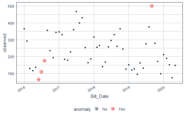
Anomaly Detection in Time Series in R

Here we can see the observed column is none other than the On_peak column and we plot it. The red dots are the outliers here. alpha_dots controls the transparency of the dots.

Step 6: To plot each of trend, seasonality and residue, along with the observed value, we can use the method plot_anomaly_decomposition() which visualize the time series decomposition with anomalies shown

R

plot_anomaly_decomposition(data_anomalized)

Output:

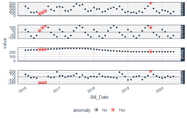
Anomaly Detection in Time Series in R

Filtering Anomalies from the Dataset

We want to get the anomalies only from the dataset, we can use the filter command along with the anomalize function used in the previous step.

Step 7: First decompose the dataset, find anomalies using anomalize, recompose it and then use the filter command. We filter based on the condition that anomaly column is true.

R

data %>%
  time_decompose(On_peak) %>%
  anomalize(remainder) %>%
  time_recompose() %>%
  filter(anomaly == 'Yes')

Output:

A time tibble: 4 × 10
Index:         Bill_Date
  Bill_Date  observed season trend remainder remainder_l1 remainder_l2 anomaly
  <date>        <dbl>  <dbl> <dbl>     <dbl>        <dbl>        <dbl> <chr>  
1 2016-06-01       63   26.1  251.     -215.        -166.         167. Yes    
2 2016-07-01      110   88.2  255.     -233.        -166.         167. Yes    
3 2016-08-01      176  131.   258.     -213.        -166.         167. Yes    
4 2019-09-01      501   95.6  203.      202.        -166.         167. Yes    
# ℹ 2 more variables: recomposed_l1 <dbl>, recomposed_l2 <dbl>

Controlling the number of Anomalies

We can also control the number of anomalies we want.

• The anomalize() method takes the following parameter to control it:
• max_anoms: The maximum percent of anomalies permitted to be identified.

Step 8: Suppose we want 25% dataset to be anomaly. So we change the value to 0.25.

R

data %>%
    time_decompose(On_peak) %>%
    anomalize(remainder, alpha = 0.75, max_anoms = 0.25) %>%
    time_recompose() %>%
    plot_anomalies(time_recomposed = TRUE) +
    ggtitle("25% Anomalies Allowed")

Output:

Anomaly Detection in Time Series in R

plot_anomalies: It is used to plot the the anomalies in one or multiple time series.

Step 9: Similarly if we want just 5%, we will provide 0.05 in max_anoms.

R

data %>%
    time_decompose(On_peak) %>%
    anomalize(remainder, alpha = 0.75, max_anoms = 0.05) %>%
    time_recompose() %>%
    plot_anomalies(time_recomposed = TRUE) +
    ggtitle("5% Anomalies Allowed ")

Output:

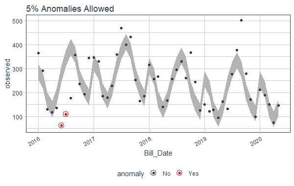
Anomaly Detection in Time Series in R

Hence we learnt to find anomalies using the anomalize package in R. We learnt to find the trends, seasonality, residue. Finally we learnt to control the percentage of anomalies in the dataset.