Machine Learning for Time Series Data in R

Machine learning (ML) is a subfield of artificial intelligence (AI) that focuses on the development of algorithms and models that enable computers to learn and make predictions or decisions without being explicitly programmed. In R Programming Language it’s a way for computers to learn from data and improve their performance on a specific task over time. Here are some key concepts in machine learning.

Time Series Data in R

Time series data is a sequence of observations or measurements collected or recorded at specific time intervals. This type of data is commonly found in various domains, including finance, economics, meteorology, and more. R provides several packages and functions to work with time series data effectively.

Time Series Components

Time series data is characterized by several key components that impact its behaviour and modelling. Understanding these components is crucial for accurate time series forecasting. The primary components are.

1. Trend: The trend component represents the long-term movement or direction in the data. It reveals the overall pattern or behaviour over an extended period. Trends can be upward, downward, or relatively stable.
2. Seasonality: Seasonality refers to periodic fluctuations or patterns that occur at regular intervals. These intervals could be daily, weekly, monthly, or yearly. For example, sales data often exhibits seasonality with higher sales during specific times of the year.
3. Cyclic Patterns: Cyclic patterns are long-term wave-like movements that are not strictly periodic like seasonality. They typically have irregular durations and amplitudes. Identifying cyclic patterns can be challenging.
4. Residuals: Residuals represent the random noise or irregular variations in the data that cannot be attributed to the trend, seasonality, or cyclic patterns. Accurate time series modelling involves minimizing these residuals.

Important steps required for Machine Learning for Time Series Data in R

Data: Machine learning algorithms require data to learn from. This data typically consists of features (input variables) and labels (output or target variables). For example, in image recognition, features might be pixel values, and labels would be the object classes.

Training: In the training phase, a machine learning model is presented with a dataset containing known inputs and outputs. The model learns to map inputs to outputs by adjusting its internal parameters.

Model: A machine learning model is a mathematical representation of a relationship between inputs and outputs. There are various types of ML models, including regression models, decision trees, neural networks, and more.

Learning: Learning refers to the process of adjusting the model’s parameters during training to minimize the difference between its predictions and the actual labels in the training data. This process is guided by a loss function that quantifies the model’s error.

Prediction: Once trained, a machine learning model can be used to make predictions or decisions on new, unseen data. It applies the learned patterns to new inputs to produce outputs or predictions.

Time Series Theory

Time series data is a type of data in which observations are collected or recorded at specific time intervals. Time series data is prevalent in various domains, including finance, economics, climate science, and more. Understanding time series data is crucial for forecasting future values or analyzing temporal patterns. Here are key concepts in time series analysis:

Time Dependency: Time series data exhibits temporal dependencies, meaning that each observation’s value depends on previous observations. This dependency can be exploited to make predictions.

Components of Time Series: Time series data can often be decomposed into three main components: trend, seasonality, and noise (random variation).

1. Trend: A long-term upward or downward movement in the data.
2. Seasonality: Repeating patterns or cycles that occur at fixed intervals.
3. Noise: Random fluctuations or unexplained variations in the data.

Stationarity: A time series is considered stationary when its statistical properties (mean, variance, etc.) remain constant over time. Many time series analysis techniques assume stationarity or require the data to be transformed to achieve it.

Modeling Techniques: Various techniques can be used to model time series data, including:

ARIMA (AutoRegressive Integrated Moving Average): A popular method for modeling stationary time series data.

Exponential Smoothing: A method for modeling time series with a trend and/or seasonality.

Prophet: An open-source forecasting tool developed by Facebook for time series data with strong seasonal patterns.

Machine Learning Models: ML algorithms, including regression, decision trees, and neural networks, can be applied to time series data for forecasting and anomaly detection.

Evaluation: Time series models are evaluated using metrics like Mean Absolute Error (MAE), Mean Squared Error (MSE), Root Mean Squared Error (RMSE), and others, depending on the specific task.

Machine learning for time series data in R involves applying various machine learning algorithms to analyze and make predictions on time-ordered data. R is a powerful programming language for statistical computing and data analysis, and it offers a wide range of packages and libraries for time series analysis and machine learning.

We have several R packages for time series analysis and machine learning. Commonly used packages include xts, zoo, forecast, tidyverse, caret, randomForest, xgboost, and keras.

Time Series Forecasting with “AirPassengers” Dataset.

R

# Load the "AirPassengers" dataset
data("AirPassengers")

# Convert the dataset to a time series object
ts_data <- ts(AirPassengers, frequency = 12, start = c(1949, 1))

# Split the data into training and testing sets
train_data <- window(ts_data, start = c(1949, 1), end = c(1958, 12))
test_data <- window(ts_data, start = c(1959, 1))

# Train an ARIMA model
arima_model <- forecast::auto.arima(train_data)
 # Forecast 12 months ahead
forecast_result <- forecast::forecast(arima_model, h = 12)

summary(arima_model)

Output:

Series: train_data 
ARIMA(1,1,0)(0,1,0)[12] 
Coefficients:
          ar1
      -0.2397
s.e.   0.0935
sigma^2 = 103.6:  log likelihood = -399.64
AIC=803.28   AICc=803.4   BIC=808.63
Training set error measures:
                      ME     RMSE      MAE         MPE    MAPE      MASE       ACF1
Training set -0.01614662 9.567988 7.120167 -0.03346415 2.90195 0.2491828 0.00821521

This line converts the loaded dataset into a time series object (ts_data). The ts() function is used to specify that the data has a monthly frequency (frequency = 12) and starts in January 1949 (start = c(1949, 1)).

Plot The Forecast

R

# Plot the forecast
plot(forecast_result, xlab = "Year", ylab = "Passenger Count",
     main = "Airline Passengers Forecast")

Output:

Airline Passengers Forecast

• The data(“AirPassengers”) command loads the built-in “AirPassengers” dataset, which contains the monthly number of airline passengers from 1949 to 1960.
• The ts_data <- ts(AirPassengers, frequency = 12, start = c(1949, 1)) line converts the loaded dataset into a time series object. The frequency argument is set to 12, indicating that the data has a monthly frequency, and the start argument specifies the starting date as January 1949.
• The train_data and test_data objects are created by using the window() function to split the time series into two parts. The training data contains observations from January 1949 to December 1958, and the testing data contains observations from January 1959 onward.
• The arima_model <- forecast::auto.arima(train_data) line trains an ARIMA (AutoRegressive Integrated Moving Average) model on the training data. The auto.arima() function automatically selects the best ARIMA model based on the data.
• The forecast_result <- forecast::forecast(arima_model, h = 12) line generates a forecast for the next 12 months using the trained ARIMA model. The h parameter specifies the number of periods (in this case, months) to forecast ahead.
• Finally, the plot() function is used to create a plot of the forecasted values. The x-axis represents the year, the y-axis represents the passenger count, and the title of the plot is set to “Airline Passengers Forecast.”

Time Series Forecasting with “Lynx Trappings” Dataset

R

# Load the package
library(forecast)
# Load the dataset
data(lynx)

# Convert data to a time series object
ts_data <- ts(lynx, frequency = 1, start = c(1821))

# Fit an ARIMA model to the data
arima_model <- auto.arima(ts_data)

# Split data into training and testing sets
train_data <- window(ts_data, start = c(1821), end = c(1900))
test_data <- window(ts_data, start = c(1901))

# Fit ARIMA model on training data
arima_model <- arima(train_data, order = arima_model$arma[c(1, 6, 2)])

# Forecast using the ARIMA model
forecast_values <- forecast(arima_model, h = length(test_data))

# Calculate RMSE to evaluate model performance
rmse <- sqrt(mean((forecast_values$mean - test_data)^2))
print(paste("Root Mean Squared Error (RMSE):", round(rmse, 2)))

# Plot the forecasted values
plot(forecast_values, main = "Annual Lynx Trappings Forecast")
lines(test_data, col = "blue")

Output:

[1] "Root Mean Squared Error (RMSE): 1698.47"

Annual Lynx Trappings Forecast

• First loads the built-in “lynx” dataset into the R environment. This dataset contains the annual number of lynx trappings, which is often used for time series analysis.
• we convert the loaded data into a time series object using the ts() function. We specify the frequency as 1 since the data is annual, and we set the start year as 1821.
• auto.arima() function from the forecast package to automatically select an appropriate ARIMA model for the time series data. The function determines the order of differencing (d) and the orders of the autoregressive (p) and moving average (q) components.
• We split the time series data into two parts: a training set (from 1821 to 1900) and a testing set (from 1901 onwards). The training set is used to fit the ARIMA model, and the testing set is used to evaluate the model’s performance.
• ARIMA model to the training data using the order parameters determined by the auto.arima() function. The chosen order parameters are based on statistical criteria and are specified in the order argument
• We use the trained ARIMA model to make forecasts for the length of the testing set, which is the number of years from 1901 onwards. The forecast() function generates the forecasted values.
• We calculate the Root Mean Squared Error (RMSE) to evaluate the accuracy of the model’s forecasts. The RMSE measures the average error of the model’s predictions compared to the actual values in the testing set.
• Finally, we create a plot that displays the forecasted values along with the actual values from the testing set, allowing us to visually assess the model’s performance.

Time Series Forecasting of Nile River Flow

R

# Load the dataset
data(Nile)

# Convert data to a time series object
ts_data <- ts(Nile, frequency = 1, start = c(1871))

# Fit an ARIMA model to the data
arima_model <- auto.arima(ts_data)

# Split data into training and testing sets
train_data <- window(ts_data, start = c(1871), end = c(1950))
test_data <- window(ts_data, start = c(1951))

# Fit ARIMA model on training data
arima_model <- arima(train_data, order = arima_model$arma[c(1, 6, 2)])

# Forecast using the ARIMA model
forecast_values <- forecast(arima_model, h = length(test_data))

# Calculate RMSE to evaluate model performance
rmse <- sqrt(mean((forecast_values$mean - test_data)^2))
print(paste("Root Mean Squared Error (RMSE):", round(rmse, 2)))

# Plot the forecasted values
plot(forecast_values, main = "Annual Nile River Flow Forecast")
lines(test_data, col = "blue")

Output:

[1] "Root Mean Squared Error (RMSE): 125.05"

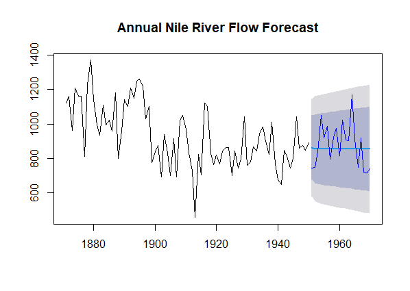
Annual Nile River Flow Forecast

First loads the built-in “Nile” dataset into the R environment. The “Nile” dataset contains annual flow data of the Nile River from 1871 to 1970.

• Here, we convert the loaded data into a time series object using the ts() function. We specify that the data is annual (frequency = 1) and set the starting year as 1871.
• auto.arima() function from the forecast package to automatically determine an appropriate ARIMA model for the time series data. It selects the orders of differencing (d) and the autoregressive (p) and moving average (q) components.
• We divide the time series data into two parts: a training set (from 1871 to 1950) and a testing set (from 1951 onwards). The training set will be used to fit the ARIMA model, while the testing set is used to evaluate the model’s forecasting accuracy.
• This line fits an ARIMA model to the training data using the order parameters determined by the auto.arima() function. The selected order parameters are based on statistical criteria and are specified in the order argument of the arima() function.
• To assess the accuracy of the model’s forecasts, we calculate the Root Mean Squared Error (RMSE). The RMSE measures the average error between the model’s predictions and the actual values in the testing set. We print the RMSE for evaluation.
• Finally, we create a plot that displays the forecasted values (in black) and overlays them with the actual values from the testing set (in blue). This visual representation helps in assessing the performance of the ARIMA model in capturing the flow pattern of the Nile River.

Conclusion

machine learning is a broader field concerned with algorithms and models capable of learning patterns and making predictions, while time series analysis focuses specifically on data collected over time, with an emphasis on understanding temporal dependencies, patterns, and forecasting future values. Machine learning techniques can be applied to time series data to build predictive models.