Random Forest for Time Series Forecasting using R

Random Forest is an ensemble machine learning method that can be used for time series forecasting. It is based on decision trees and combines multiple decision trees to make more accurate predictions. Here’s a complete explanation along with an example of using Random Forest for time series forecasting in R.

Time Series Forecasting

Time series forecasting is a crucial component of data analysis and predictive modelling. It involves predicting future values based on historical time-ordered data. In the R Programming Language, there are several libraries and techniques available for time series forecasting. Here’s a high-level overview of the theory behind time series forecasting using R.

Time Series Data

• Time series data is a sequence of observations or measurements collected or recorded at specific time intervals. Examples include stock prices, weather data, sales figures, and more.
• In R, time series data is often stored in objects like “ts” (time series) or “xts” (extensible time series) for efficient handling.

Components of Time Series

Time series data typically comprises three main components:

• Trend: The long-term movement or direction in the data. It represents the general pattern or behaviour.
• Seasonality: Periodic fluctuations or patterns that occur at regular intervals. These cycles could be daily, weekly, monthly, or annual. Identifying and modelling seasonality is crucial in time series analysis.
• Residuals: These are random fluctuations or irregular variations that cannot be attributed to the trend or seasonality. Residuals represent the noise in the data.

Random Forest for time series forecasting

Random Forest is one of the main machine learning techniques and we use this for time series forecasting.

Data Preparation

• Convert your time series data into a suitable format. In R, the “xts” package is often used to work with time series data.
• Create lag features to capture temporal patterns. These lags represent previous values of the time series, and they are used as predictor variables.

Data Splitting

• Divide our data into training and testing sets. The training set contains historical data, and the testing set contains the future data that you want to forecast.
• Ensure that the time order is preserved to avoid data leakage.

Model Building

• Fit a Random Forest model to the training data using the randomForest function.
• Specify the response variable (the value you want to forecast) and predictor variables, which include lag features and other relevant information.
• Random Forest is an ensemble method that combines multiple decision trees to make predictions. Each tree is trained on a bootstrapped sample of the data and a random subset of predictor variables.

Prediction

• Use the trained Random Forest model to make predictions on the testing data.
• The model will provide forecasts for future time points based on the historical data.

Model Evaluation

• Evaluate the model’s performance using appropriate metrics, such as Mean Absolute Error (MAE), Mean Squared Error (MSE), or Root Mean Squared Error (RMSE).
• These metrics help assess the accuracy and reliability of the forecasts.

Visualization

Visualize the original time series data along with the forecasted values. Plotting the actual and predicted values on the same graph can provide insights into the model’s accuracy and how it captures trends and seasonality.

Here’s a complete example using the “AirPassengers” dataset

R

# Load required libraries
library(randomForest)
library(xts)
library(ggplot2)

# Load the AirPassengers dataset
data("AirPassengers")
ts_data <- AirPassengers

# Convert the time series to a data frame
ts_df <- data.frame(Date = index(ts_data), Passengers = coredata(ts_data))

# Convert Date to a time series object
ts_df$Date <- as.Date(ts_df$Date)
ts_xts <- xts(ts_df$Passengers, order.by = ts_df$Date)

# Create lag features for time series data
lags <- 1:12  # Number of lags to consider
lagged_data <- lag(ts_xts, k = lags)  # Create lagged data

# Combine the lagged features into one data frame
lagged_df <- data.frame(lagged_data)
colnames(lagged_df) <- paste0("lag_", lags)  # Rename columns with lag prefixes

# Merge the lagged features with the original data
final_data <- cbind(ts_df, lagged_df)  # Combine data frames

# Remove rows with NAs created by lagging
final_data <- final_data[complete.cases(final_data), ]

# Split the data into training and testing sets
train_percentage <- 0.8
train_size <- floor(train_percentage * nrow(final_data))
train_data <- final_data[1:train_size, ]
test_data <- final_data[(train_size + 1):nrow(final_data), ]

# Fit a Random Forest model
rf_model <- randomForest(Passengers ~ ., data = train_data, ntree = 100)

# Make predictions on the test data
predictions <- predict(rf_model, newdata = test_data)

# Evaluate the model using RMSE
rmse <- sqrt(mean((test_data$Passengers - predictions)^2))
cat("RMSE:", rmse, "\n")

Output:

RMSE: 57.30901 

The required libraries, including randomForest for Random Forest modeling, xts for time series data, and ggplot2 for data visualization, are loaded.

• The “AirPassengers” dataset is loaded, which contains monthly airline passenger counts.
• The time series data is converted into a data frame, making it suitable for further manipulation and modeling.
• Lag features are created for the time series data. The code creates lagged versions of the passenger counts from 1 to 12 months ago, effectively capturing historical values as features.
• The lagged features are combined into a new data frame called “lagged_df,” and the columns are named with “lag_” prefixes.
• The lagged features are merged with the original data to create the “final_data” data frame.
• Rows with missing values created by lagging are removed to ensure that the dataset is clean.
• The data is split into training and testing sets. In this code, 80% of the data is used for training the model, and the remaining 20% is used for testing.
• A Random Forest model is trained using the randomForest function. The model is fitted to predict the “Passengers” variable based on the lagged features and other attributes in the training data. ntree specifies the number of trees in the forest (100 in this case).
• Predictions are made on the test data using the trained Random Forest model.
• The model’s performance is evaluated using the Root Mean Squared Error (RMSE), which measures the accuracy of the model’s predictions. A lower RMSE indicates better model performance.

Plot the original time series and the forecast

R

# Plot the original time series and the forecast
ggplot(final_data) +
  geom_line(aes(x = Date, y = Passengers, color = "Original")) +
  geom_line(data = test_data, aes(x = Date, y = predictions, color = "Forecast")) +
  scale_color_manual(values = c("Original" = "blue", "Forecast" = "red")) +
  labs(title = "Time Series Forecasting with Random Forest", y = "Passengers")

Output:

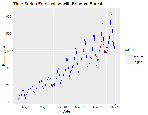
Random Forest for Time Series Forecasting using R

We added to the plot using the geom_line function. It specifies that the x-axis is represented by the “Date” column, and the y-axis is represented by the “Passengers” column. The color aesthetic is set to “Original,” which assigns a blue color to the line representing the original time series data.

• Another line is added to the plot, this time using data from the “test_data” data frame. It represents the forecasted values produced by the Random Forest model. The x-axis is still “Date,” and the y-axis is “predictions.” The color aesthetic is set to “Forecast,” assigning a red color to this line.
• This line customizes the color scale for the lines in the plot. It specifies that “Original” should be blue, and “Forecast” should be red.
• Finally, the labs function is used to set the plot’s title to “Time Series Forecasting with Random Forest” and label the y-axis as “Passengers.”

Conclusion

The Random Forest model’s performance can be assessed by examining the RMSE and by visually inspecting the chart. A lower RMSE suggests that the model is making more accurate predictions. The visualization allows for a qualitative assessment of the model’s ability to capture patterns and trends in the time series data.

Time series forecasting with Random Forest can be a powerful technique when you need to predict future values based on historical data. It is essential to preprocess the data, choose appropriate features, and carefully evaluate the model’s performance to ensure accurate and reliable forecasts.