Time Series Forecasting using Recurrent Neural Networks (RNN) in TensorFlow

Time Series Data: Each data point in a time series is linked to a timestamp, which shows the exact time when the data was observed or recorded. Many fields, including finance, economics, weather forecasting, and machine learning, frequently employ this kind of data.

The fact that time series data frequently display patterns or trends across time, such as seasonality or cyclical patterns, is an essential feature associated with it. To make predictions or learn more about the underlying processes or occurrences being observed, these patterns can be analyzed and modeled.

Recurrent Neural Networks (RNN) model the temporal dependencies present in the data as it contains an implicit memory of previous inputs. Hence, time series data being sequential in nature is often used in RNN. For working with time series data in RNNs, TensorFlow provides a number of APIs and tools, like tf.keras.layers.RNN API, which allows to create of unique RNN cell classes and use them with data. Several RNN cell types are also supported by this API, including Basic RNN, LSTM, and GRU. 

To demonstrate the same, we’re going the run the following code snippets in Google Colaboratory which comes pre-installed with Machine Learning and Deep Learning Libraries. This example will use stock price data, the most popular type of time series data.

Step 1: Import the required libraries.

• Numpy & Pandas – For data manipulation and analysis
• Matplotlib – For data visualization.
• Yahoo Finance – Provides financial data for analysis.
• Datetime – For working with dates and times.
• Math – Provides basic mathematical functions in Python.

Python3

import numpy as np
import pandas as pd
import yfinance as yf
import datetime as dt
import matplotlib.pyplot as plt
import math

Step 2: This code uses the yf.download() method of the yfinance library to download historical stock data for Google from Yahoo Finance. Using the dt.datetime() method of the datetime module, the start and end dates of the time period for which the data has been obtained are given.

The downloaded data is then shown using the print() function, where the Pandas DataFrame’s display options are configured using pd.set_option().

Python3

#the start and end date
start_date = dt.datetime(2020,4,1)
end_date = dt.datetime(2023,4,1)

#loading from yahoo finance
data = yf.download("GOOGL",start_date, end_date)

pd.set_option('display.max_rows', 4)
pd.set_option('display.max_columns',5)
print(data)

Output:

[*********************100%***********************]  1 of 1 completed
                  Open        High  ...   Adj Close    Volume
Date                                ...                      
2020-04-01   56.200001   56.471001  ...   55.105000  51970000
2020-04-02   55.000000   56.138500  ...   55.851501  56410000
...                ...         ...  ...         ...       ...
2023-03-30  100.910004  101.160004  ...  100.889999  33086200
2023-03-31  101.300003  103.889999  ...  103.730003  36823200

[756 rows x 6 columns]

Step 3: Next, we split the dataset into training and testing in the ratio 80:20. Only the first column of the data is chosen using iloc[:,:1] and the train_data contains the first training_data_len rows of the original data. The test_data, contains all of the remaining rows of the original data starting from training_data_len to the end.

Python3

# Setting 80 percent data for training
training_data_len = math.ceil(len(data) * .8)
training_data_len

#Splitting the dataset
train_data = data[:training_data_len].iloc[:,:1]
test_data = data[training_data_len:].iloc[:,:1]
print(train_data.shape, test_data.shape)

 Output:

(605, 1) (151, 1)

Step 4: This code creates a numpy array called dataset_train and populates it with the “Open” pricing values from the training data. The 1-dimensional array is then transformed into a 2-dimensional array. The shape property, which returns the tuple (num_rows, num_columns) denoting the dataset_train array’s final shape.

Python3

# Selecting Open Price values
dataset_train = train_data.Open.values
# Reshaping 1D to 2D array
dataset_train = np.reshape(dataset_train, (-1,1))
dataset_train.shape

Output:

(605, 1)

Step 5: Normalization is a crucial step in data preprocessing to enhance the effectiveness and interpretability of machine learning models. Hence MinMaxScaler from sklearn is imported to scale the dataset from 0 to 1. Using the sklearn fit_transform() method, the training dataset is scaled.

Python3

from sklearn.preprocessing import MinMaxScaler
scaler = MinMaxScaler(feature_range=(0,1))
# scaling dataset
scaled_train = scaler.fit_transform(dataset_train)

print(scaled_train[:5])

Output:

[[0.01246754]
 [0.        ]
 [0.00764156]
 [0.01714287]
 [0.0607844 ]]

Step 6: The same data preprocessing is done for test data.

Python3

# Selecting Open Price values
dataset_test = test_data.Open.values
# Reshaping 1D to 2D array
dataset_test = np.reshape(dataset_test, (-1,1))
# Normalizing values between 0 and 1
scaled_test = scaler.fit_transform(dataset_test)
print(*scaled_test[:5])

Output:

[0.98362881] [1.] [0.83867656] [0.84481572] [0.86118691]

Step 7: The time-series data must be divided into X_train and y_train from the training set and X_test and y_test from the testing set in this phase. It is done to turn time series data into a supervised learning problem that can be utilized to train the model. The loop generates input/output sequences of length 50 while iterating through the time series data. Using this method, we can forecast future values while taking into consideration the data’s temporal dependence on prior observations.

For training set:

Python3

X_train = []
y_train = []
for i in range(50, len(scaled_train)):
    X_train.append(scaled_train[i-50:i, 0])
    y_train.append(scaled_train[i, 0])
    if i <= 51:
        print(X_train)
        print(y_train)
        print()

Output:

[array([0.01246754, 0.        , 0.00764156, 0.01714287, 0.0607844 ,
       0.05355843, 0.06139221, 0.05272728, 0.0727117 , 0.0761091 ,
       0.08682596, 0.0943896 , 0.08825454, 0.07413508, 0.0733039 ,
       0.08609869, 0.08051948, 0.09974024, 0.09516887, 0.12727273,
       0.12018702, 0.11641037, 0.1081195 , 0.12337662, 0.13402599,
       0.13574544, 0.14640004, 0.14378702, 0.16011432, 0.14345973,
       0.12130912, 0.12896625, 0.13588574, 0.14830132, 0.15021299,
       0.16155324, 0.15787013, 0.17764155, 0.16623377, 0.15584416,
       0.16645714, 0.16919484, 0.17402597, 0.178026  , 0.17495062,
       0.16396881, 0.16949613, 0.17934547, 0.18779741, 0.17715843])]
[0.16927791446834417]

[array([0.01246754, 0.        , 0.00764156, 0.01714287, 0.0607844 ,
       0.05355843, 0.06139221, 0.05272728, 0.0727117 , 0.0761091 ,
       0.08682596, 0.0943896 , 0.08825454, 0.07413508, 0.0733039 ,
       0.08609869, 0.08051948, 0.09974024, 0.09516887, 0.12727273,
       0.12018702, 0.11641037, 0.1081195 , 0.12337662, 0.13402599,
       0.13574544, 0.14640004, 0.14378702, 0.16011432, 0.14345973,
       0.12130912, 0.12896625, 0.13588574, 0.14830132, 0.15021299,
       0.16155324, 0.15787013, 0.17764155, 0.16623377, 0.15584416,
       0.16645714, 0.16919484, 0.17402597, 0.178026  , 0.17495062,
       0.16396881, 0.16949613, 0.17934547, 0.18779741, 0.17715843]), 
array([0.        , 0.00764156, 0.01714287, 0.0607844 , 0.05355843,
       0.06139221, 0.05272728, 0.0727117 , 0.0761091 , 0.08682596,
       0.0943896 , 0.08825454, 0.07413508, 0.0733039 , 0.08609869,
       0.08051948, 0.09974024, 0.09516887, 0.12727273, 0.12018702,
       0.11641037, 0.1081195 , 0.12337662, 0.13402599, 0.13574544,
       0.14640004, 0.14378702, 0.16011432, 0.14345973, 0.12130912,
       0.12896625, 0.13588574, 0.14830132, 0.15021299, 0.16155324,
       0.15787013, 0.17764155, 0.16623377, 0.15584416, 0.16645714,
       0.16919484, 0.17402597, 0.178026  , 0.17495062, 0.16396881,
       0.16949613, 0.17934547, 0.18779741, 0.17715843, 0.16927791])]
[0.16927791446834417, 0.15038444221793834]

For testing set:

Python3

X_test = []
y_test = []
for i in range(50, len(scaled_test)):
    X_test.append(scaled_test[i-50:i, 0])
    y_test.append(scaled_test[i, 0])

Step 8: In this step, the data is converted into a format that is suitable for input to an RNN. np.reshape(X_train, (X_train.shape[0], X_train.shape[1], 1)) transforms the X_train array, which was originally a 2-dimensional array of shape (samples, features), into a 3-dimensional array of shape (samples, time steps, features), where time steps denotes the number of time steps in the input sequence and features denotes the number of features in the input data. Size 1 is an additional dimension that serves as an indication that each time step only has a single feature.

The y_train array is transformed from a 1-dimensional array of shape (samples) into a 2-dimensional array of shape (samples, 1) by np.reshape(y_train, (y_train.shape[0], 1)), where each row represents the output value at a certain time step. 

For training set:

Python3

# The data is converted to Numpy array
X_train, y_train = np.array(X_train), np.array(y_train)

#Reshaping
X_train = np.reshape(X_train, (X_train.shape[0], X_train.shape[1],1))
y_train = np.reshape(y_train, (y_train.shape[0],1))
print("X_train :",X_train.shape,"y_train :",y_train.shape)

Output:

X_train : (555, 50, 1) y_train : (555, 1)

For testing set:

Python3

# The data is converted to numpy array
X_test, y_test = np.array(X_test), np.array(y_test)

#Reshaping
X_test = np.reshape(X_test, (X_test.shape[0], X_test.shape[1],1))
y_test = np.reshape(y_test, (y_test.shape[0],1))
print("X_test :",X_test.shape,"y_test :",y_test.shape)

Output:

X_test : (101, 50, 1) y_test : (101, 1)

Step 9: Three RNN models are created in this step. The libraries needed for the model is imported.

Python3

# importing libraries
from keras.models import Sequential
from keras.layers import LSTM
from keras.layers import Dense
from keras.layers import SimpleRNN
from keras.layers import Dropout
from keras.layers import GRU, Bidirectional
from keras.optimizers import SGD
from sklearn import metrics
from sklearn.metrics import mean_squared_error

SimpleRNN Model: 

Using the Keras API, this code creates a recurrent neural network (RNN) with four layers of basic RNNs and a dense output layer. It makes use of the tanh hyperbolic tangent activation function. To avoid overfitting, a dropout layer with a rate of 0.2 is introduced. It employs the optimizer as Adam, mean squared error as the loss function, and accuracy as the evaluation metric while compiling. With a batch size of 2, it fits the model to the training data for 20 epochs. The number of parameters in each layer and the overall number of parameters in the model are listed in a summary of the model architecture.

Python3

# initializing the RNN
regressor = Sequential()

# adding RNN layers and dropout regularization
regressor.add(SimpleRNN(units = 50,
                        activation = "tanh",
                        return_sequences = True,
                        input_shape = (X_train.shape[1],1)))
regressor.add(Dropout(0.2))

regressor.add(SimpleRNN(units = 50,
                        activation = "tanh",
                        return_sequences = True))

regressor.add(SimpleRNN(units = 50,
                        activation = "tanh",
                        return_sequences = True))

regressor.add( SimpleRNN(units = 50))

# adding the output layer
regressor.add(Dense(units = 1,activation='sigmoid'))

# compiling RNN
regressor.compile(optimizer = SGD(learning_rate=0.01,
                                  decay=1e-6,
                                  momentum=0.9,
                                  nesterov=True),
                  loss = "mean_squared_error")

# fitting the model
regressor.fit(X_train, y_train, epochs = 20, batch_size = 2)
regressor.summary()

Output:

Epoch 1/20
278/278 [==============================] - 13s 39ms/step - loss: 0.0187
Epoch 2/20
278/278 [==============================] - 11s 39ms/step - loss: 0.0035
Epoch 3/20
278/278 [==============================] - 11s 39ms/step - loss: 0.0031
Epoch 4/20
278/278 [==============================] - 12s 42ms/step - loss: 0.0028
Epoch 5/20
278/278 [==============================] - 11s 39ms/step - loss: 0.0027
Epoch 6/20
278/278 [==============================] - 10s 36ms/step - loss: 0.0023
Epoch 7/20
278/278 [==============================] - 11s 39ms/step - loss: 0.0026
Epoch 8/20
278/278 [==============================] - 11s 39ms/step - loss: 0.0023
Epoch 9/20
278/278 [==============================] - 11s 39ms/step - loss: 0.0021
Epoch 10/20
278/278 [==============================] - 11s 40ms/step - loss: 0.0021
Epoch 11/20
278/278 [==============================] - 11s 39ms/step - loss: 0.0019
Epoch 12/20
278/278 [==============================] - 11s 39ms/step - loss: 0.0019
Epoch 13/20
278/278 [==============================] - 11s 39ms/step - loss: 0.0022
Epoch 14/20
278/278 [==============================] - 11s 39ms/step - loss: 0.0019
Epoch 15/20
278/278 [==============================] - 11s 39ms/step - loss: 0.0019
Epoch 16/20
278/278 [==============================] - 11s 39ms/step - loss: 0.0018
Epoch 17/20
278/278 [==============================] - 10s 36ms/step - loss: 0.0019
Epoch 18/20
278/278 [==============================] - 11s 39ms/step - loss: 0.0017
Epoch 19/20
278/278 [==============================] - 11s 39ms/step - loss: 0.0016
Epoch 20/20
278/278 [==============================] - 11s 39ms/step - loss: 0.0016
Model: "sequential_6"
_________________________________________________________________
 Layer (type)                Output Shape              Param #   
=================================================================
 simple_rnn_24 (SimpleRNN)   (None, 50, 50)            2600      
                                                                 
 dropout_6 (Dropout)         (None, 50, 50)            0         
                                                                 
 simple_rnn_25 (SimpleRNN)   (None, 50, 50)            5050      
                                                                 
 simple_rnn_26 (SimpleRNN)   (None, 50, 50)            5050      
                                                                 
 simple_rnn_27 (SimpleRNN)   (None, 50)                5050      
                                                                 
 dense_6 (Dense)             (None, 1)                 51        
                                                                 
=================================================================
Total params: 17,801
Trainable params: 17,801
Non-trainable params: 0
_________________________________________________________________

LSTM RNN Model:  

This code creates a LSTM Model with three layers and a dense output layer. It employs the optimizer as Adam, mean squared error as the loss function, and accuracy as the evaluation metric while compiling. With a batch size of 1, it fits the model to the training data for 10 epochs. The number of parameters in each layer and the overall number of parameters in the model are listed in a summary of the model architecture.

Python3

#Initialising the model
regressorLSTM = Sequential()

#Adding LSTM layers
regressorLSTM.add(LSTM(50,
                       return_sequences = True,
                       input_shape = (X_train.shape[1],1)))
regressorLSTM.add(LSTM(50,
                       return_sequences = False))
regressorLSTM.add(Dense(25))

#Adding the output layer
regressorLSTM.add(Dense(1))

#Compiling the model
regressorLSTM.compile(optimizer = 'adam',
                      loss = 'mean_squared_error',
                      metrics = ["accuracy"])

#Fitting the model
regressorLSTM.fit(X_train,
                  y_train,
                  batch_size = 1,
                  epochs = 12)
regressorLSTM.summary()

Output:

Epoch 1/12
555/555 [==============================] - 18s 25ms/step - loss: 0.0050
Epoch 2/12
555/555 [==============================] - 14s 25ms/step - loss: 0.0024
Epoch 3/12
555/555 [==============================] - 14s 25ms/step - loss: 0.0018
Epoch 4/12
555/555 [==============================] - 14s 25ms/step - loss: 0.0017
Epoch 5/12
555/555 [==============================] - 14s 25ms/step - loss: 0.0013
Epoch 6/12
555/555 [==============================] - 14s 25ms/step - loss: 0.0013
Epoch 7/12
555/555 [==============================] - 14s 26ms/step - loss: 0.0010
Epoch 8/12
555/555 [==============================] - 14s 25ms/step - loss: 0.0010
Epoch 9/12
555/555 [==============================] - 14s 25ms/step - loss: 9.8315e-04
Epoch 10/12
555/555 [==============================] - 15s 26ms/step - loss: 0.0011
Epoch 11/12
555/555 [==============================] - 14s 25ms/step - loss: 0.0011
Epoch 12/12
555/555 [==============================] - 14s 24ms/step - loss: 9.1305e-04
Model: "sequential_15"
_________________________________________________________________
 Layer (type)                Output Shape              Param #   
=================================================================
 lstm_12 (LSTM)              (None, 50, 50)            10400     
                                                                 
 lstm_13 (LSTM)              (None, 50)                20200     
                                                                 
 dense_19 (Dense)            (None, 25)                1275      
                                                                 
 dense_20 (Dense)            (None, 1)                 26        
                                                                 
=================================================================
Total params: 31,901
Trainable params: 31,901
Non-trainable params: 0
_________________________________________________________________

GRU RNN Model: 

This code defines a recurrent neural network (RNN) model using the GRU (Gated Recurrent Unit) layer in Keras. It consists of four stacked GRU layers followed by a single output layer. It makes use of the ‘tanh’ hyperbolic tangent activation function. To avoid overfitting, a dropout layer with a rate of 0.2 is introduced. It employs the optimizer as Stochastic Gradient Descent (SGD) with a learning rate of 0.01, the decay rate of 1e-7, the momentum of 0.9, and Nesterov is set to False. The mean squared error is the loss function, and accuracy is the evaluation metric while compiling. With a batch size of 2, it fits the model to the training data for 20 epochs. The number of parameters in each layer and the overall number of parameters in the model are listed in a summary of the model architecture.

Python3

#Initialising the model
regressorGRU = Sequential()

# GRU layers with Dropout regularisation
regressorGRU.add(GRU(units=50,
                     return_sequences=True,
                     input_shape=(X_train.shape[1],1),
                     activation='tanh'))
regressorGRU.add(Dropout(0.2))

regressorGRU.add(GRU(units=50,
                     return_sequences=True,
                     activation='tanh'))

regressorGRU.add(GRU(units=50,
                     return_sequences=True,
                     activation='tanh'))

regressorGRU.add(GRU(units=50,
                     activation='tanh'))

# The output layer
regressorGRU.add(Dense(units=1,
                       activation='relu'))
# Compiling the RNN
regressorGRU.compile(optimizer=SGD(learning_rate=0.01,
                                   decay=1e-7,
                                   momentum=0.9,
                                   nesterov=False),
                     loss='mean_squared_error')

# Fitting the data
regressorGRU.fit(X_train,y_train,epochs=20,batch_size=1)
regressorGRU.summary()

Output:

Epoch 1/20
555/555 [==============================] - 32s 46ms/step - loss: 0.0155
Epoch 2/20
555/555 [==============================] - 26s 46ms/step - loss: 0.0027
Epoch 3/20
555/555 [==============================] - 26s 46ms/step - loss: 0.0030
Epoch 4/20
555/555 [==============================] - 26s 46ms/step - loss: 0.0026
Epoch 5/20
555/555 [==============================] - 26s 47ms/step - loss: 0.0022
Epoch 6/20
555/555 [==============================] - 26s 48ms/step - loss: 0.0025
Epoch 7/20
555/555 [==============================] - 26s 46ms/step - loss: 0.0021
Epoch 8/20
555/555 [==============================] - 26s 46ms/step - loss: 0.0021
Epoch 9/20
555/555 [==============================] - 25s 46ms/step - loss: 0.0021
Epoch 10/20
555/555 [==============================] - 27s 49ms/step - loss: 0.0021
Epoch 11/20
555/555 [==============================] - 27s 49ms/step - loss: 0.0022
Epoch 12/20
555/555 [==============================] - 27s 48ms/step - loss: 0.0022
Epoch 13/20
555/555 [==============================] - 28s 50ms/step - loss: 0.0022
Epoch 14/20
555/555 [==============================] - 28s 50ms/step - loss: 0.0021
Epoch 15/20
555/555 [==============================] - 26s 48ms/step - loss: 0.0018
Epoch 16/20
555/555 [==============================] - 27s 48ms/step - loss: 0.0021
Epoch 17/20
555/555 [==============================] - 27s 49ms/step - loss: 0.0021
Epoch 18/20
555/555 [==============================] - 26s 47ms/step - loss: 0.0019
Epoch 19/20
555/555 [==============================] - 27s 48ms/step - loss: 0.0019
Epoch 20/20
555/555 [==============================] - 27s 48ms/step - loss: 0.0018
Model: "sequential_17"
_________________________________________________________________
 Layer (type)                Output Shape              Param #   
=================================================================
 gru_4 (GRU)                 (None, 50, 50)            7950      
                                                                 
 dropout_8 (Dropout)         (None, 50, 50)            0         
                                                                 
 gru_5 (GRU)                 (None, 50, 50)            15300     
                                                                 
 gru_6 (GRU)                 (None, 50, 50)            15300     
                                                                 
 gru_7 (GRU)                 (None, 50)                15300     
                                                                 
 dense_22 (Dense)            (None, 1)                 51        
                                                                 
=================================================================
Total params: 53,901
Trainable params: 53,901
Non-trainable params: 0
_________________________________________________________________

Step 10: The X_test data is then used to make predictions from all three models.

Python3

# predictions with X_test data
y_RNN = regressor.predict(X_test)
y_LSTM = regressorLSTM.predict(X_test)
y_GRU = regressorGRU.predict(X_test)

Step 11:  The predicted values are transformed back from the normalized state to their original scale using the inverse_transform() function.

Python3

# scaling back from 0-1 to original
y_RNN_O = scaler.inverse_transform(y_RNN)
y_LSTM_O = scaler.inverse_transform(y_LSTM)
y_GRU_O = scaler.inverse_transform(y_GRU)

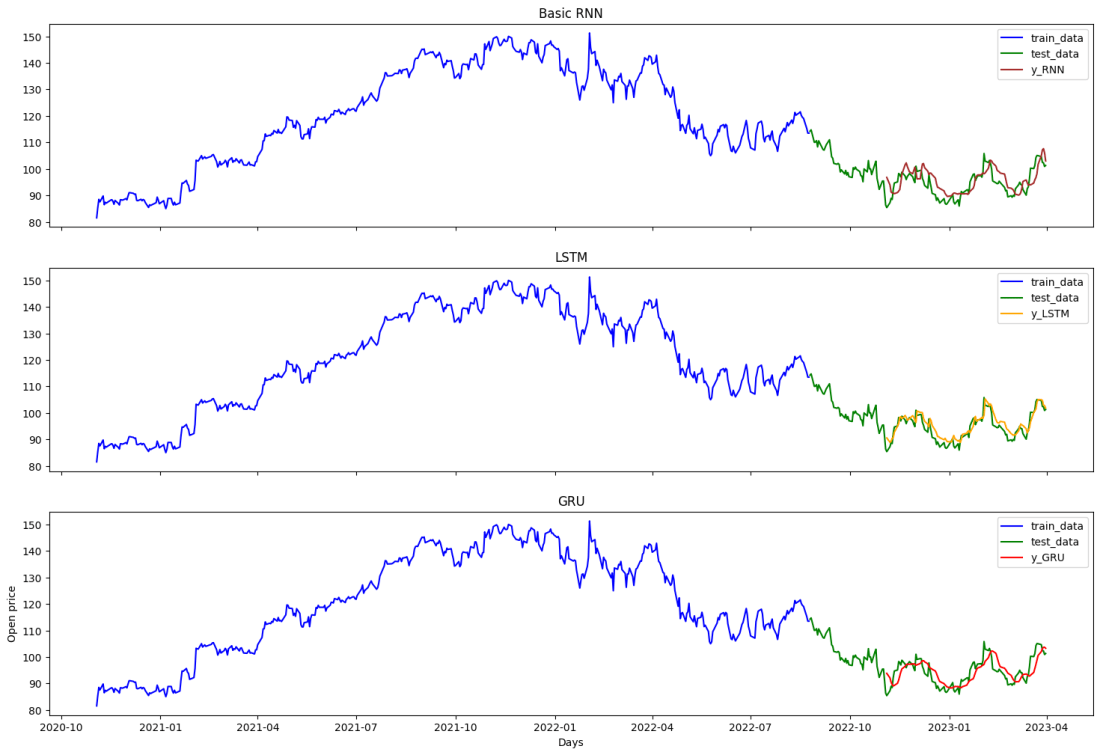
Step 12: Visualize the predicted prices using matplotlib.

Python3

fig, axs = plt.subplots(3,figsize =(18,12),sharex=True, sharey=True)
fig.suptitle('Model Predictions')

#Plot for RNN predictions
axs[0].plot(train_data.index[150:], train_data.Open[150:], label = "train_data", color = "b")
axs[0].plot(test_data.index, test_data.Open, label = "test_data", color = "g")
axs[0].plot(test_data.index[50:], y_RNN_O, label = "y_RNN", color = "brown")
axs[0].legend()
axs[0].title.set_text("Basic RNN")

#Plot for LSTM predictions
axs[1].plot(train_data.index[150:], train_data.Open[150:], label = "train_data", color = "b")
axs[1].plot(test_data.index, test_data.Open, label = "test_data", color = "g")
axs[1].plot(test_data.index[50:], y_LSTM_O, label = "y_LSTM", color = "orange")
axs[1].legend()
axs[1].title.set_text("LSTM")

#Plot for GRU predictions
axs[2].plot(train_data.index[150:], train_data.Open[150:], label = "train_data", color = "b")
axs[2].plot(test_data.index, test_data.Open, label = "test_data", color = "g")
axs[2].plot(test_data.index[50:], y_GRU_O, label = "y_GRU", color = "red")
axs[2].legend()
axs[2].title.set_text("GRU")

plt.xlabel("Days")
plt.ylabel("Open price")

plt.show()

Output:

Time Series Forecasting