What is a trend in time series?

Time series data is a sequence of data points that measure some variable over ordered period of time. It is the fastest-growing category of databases as it is widely used in a variety of industries to understand and forecast data patterns. So while preparing this time series data for modeling it’s important to check for time series components or patterns.  One of these components is Trend. 

Trend is a pattern in data that shows the movement of a series to relatively higher or lower values over a long period of time. In other words, a trend is observed when there is an increasing or decreasing slope in the time series. Trend usually happens for some time and then disappears, it does not repeat. For example, some new song comes, it goes trending for a while, and then disappears. There is fairly any chance that it would be trending again.

A trend could be :

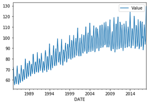
• Uptrend: Time Series Analysis shows a general pattern that is upward then it is Uptrend.
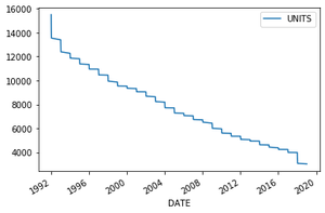
• Downtrend: Time Series Analysis shows a pattern that is downward then it is Downtrend.
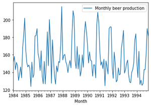
• Horizontal or Stationary trend: If no pattern observed then it is called a Horizontal or stationary trend.

You can find trends in data either by simply visualizing or by the decomposing dataset.

Visualization

By simply plotting the dataset you can see the general trend in data

Approach :  

• Import module
• Load dataset
• Cast month column to date time object
• Set month as index
• Create plot

Note: In the examples given below the same code is used to show all three trends just the dataset used is different to reflect that particular trend.

Example: Uptrend 

Python3

# importing the libraries
import pandas as pd
import matplotlib

# importing dataset
data = pd.read_csv(r'C:\Users\admin\Downloads\Electric_Production.csv')

# casting Month column to datetime object
data['DATE'] = pd.to_datetime(data['DATE'])

# Setting Month as index
data = data.set_index('DATE')

# Creating the plot
data.plot()

Output : 

Example: Downtrend

Python3

import pandas as pd
import matplotlib

# importing dataset
data = pd.read_csv(r'C:\Users\admin\Downloads\AlcoholSale.csv')

# casting Date column to datetime object
data['DATE'] = pd.to_datetime(data['DATE'])

# Setting Date column as index
data = data.set_index('DATE')

# Creating the plot
data.plot()

Output : 

Example: Horizontal trend

Python3

# importing the libraries
import pandas as pd
import matplotlib

# importing dataset
data = pd.read_csv(
    r'C:\Users\admin\Downloads\monthly-beer-production-in-austr.csv')

# casting Month column to datetime object
data['Month'] = pd.to_datetime(data['Month'])

# Setting Month as index
data = data.set_index('Month')

# Creating the plot
data['1984':'1994'].plot()

Output : 

Decomposition

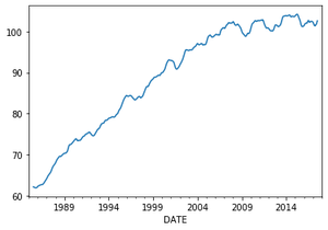
To see the complexity behind linear visualization we can decompose the data. The function called seasonal_decompose within the statsmodels package can help us to decompose the data into its components/show patterns — trend, seasonality and residual components of time series. Here we are interested in trend component only so will access it using seasonal_decompose().trend .

seasonal_decompose function uses moving averages method to estimate the trend.

Syntax : 

statsmodels.tsa.seasonal.seasonal_decompose(x, model=’additive’, period=None, extrapolate_trend=0)

Important parameters :

• x : array-like.  Time-Series.  If 2d, individual series are in columns. x must contain 2 complete cycles.
• model : {“additive”, “multiplicative”}, optional (Depends on nature on seasonal component)
• period(freq.) : int, optional . Must be use if x is not pandas object or index of  x does not have a frequency.

Returns : A object with seasonal, trend, and resid attributes.

Example : 

Python3

# importing function
from statsmodels.tsa.seasonal import seasonal_decompose

# creating trend object by assuming multiplicative model
output = seasonal_decompose(data, model='multiplicative').trend

# creating plot
output.plot()

Output :