Autoregressive (AR) Model for Time Series Forecasting

Autoregressive models, often abbreviated as AR models, are a fundamental concept in time series analysis and forecasting. They have widespread applications in various fields, including finance, economics, climate science, and more. In this comprehensive guide, we will explore autoregressive models, how they work, their types, and practical examples.

Autoregressive Models

Autoregressive models belong to the family of time series models. These models capture the relationship between an observation and several lagged observations (previous time steps). The core idea is that the current value of a time series can be expressed as a linear combination of its past values, with some random noise.

Mathematically, an autoregressive model of order p, denoted as AR(p), can be expressed as:

Where:

• is the value at time t.

• c is a constant.

• are the model parameters.

• are the lagged values.

• represents white noise (random error) at time t.

Autocorrelation (ACF) in Autoregressive Models

Autocorrelation, often denoted as “ACF” (Autocorrelation Function), is a fundamental concept in time series analysis and autoregressive models. It refers to the correlation between a time series and a lagged version of itself. In the context of autoregressive models, autocorrelation measures how closely the current value of a time series is related to its past values, specifically those at different time lags.

Here’s a breakdown of the concept of autocorrelation in autoregressive models:

• Autocorrelation involves calculating the correlation between a time series and a lagged version of itself. The “lag” represents the number of time units by which the series is shifted. For example, a lag of 1 corresponds to comparing the series with its previous time step, while a lag of 2 compares it with the time step before that, and so on. Lag values help you calculate autocorrelation, which measures how each observation in a time series is related to previous observations.
• The autocorrelation at a particular lag provides insights into the temporal dependence of the data. If the autocorrelation is high at a certain lag, it indicates a strong relationship between the current value and the value at that lag. Conversely, if the autocorrelation is low or close to zero, it suggests a weak or no relationship.
• To visualize autocorrelation, a common approach is to create an ACF plot. This plot displays the autocorrelation coefficients at different lags. The horizontal axis represents the lag, and the vertical axis represents the autocorrelation values. Significant peaks or patterns in the ACF plot can reveal the underlying temporal structure of the data. Autocorrelation plays a pivotal role in autoregressive models.
• In an Autoregressive model of order p, the current value of the time series is expressed as a linear combination of its past p values, with coefficients determined through methods like least squares or maximum likelihood estimation. The selection of the lag order (p) in the AR model often relies on the analysis of the ACF plot.
• Autocorrelation can also be used to assess whether a time series is stationary. In a stationary time series, autocorrelation should gradually decrease as the lag increases. Deviations from this behavior might indicate non-stationarity.

Types of Autoregressive Models

AR(1) Model:

• In the AR(1) model, the current value depends only on the previous value.
• It is expressed as:

AR(p) Model:

• The general autoregressive model of order p includes p lagged values.
• It is expressed as shown in the introduction.

Implementing AR Model for predicting Temperature

Step 1: Importing Data

In the first step, we import the required libraries and the temperature dataset.

Python

import pandas as pd
import numpy as np
import matplotlib.pyplot as plt


# Set a random seed for reproducibility
np.random.seed(0)

# Load your temperature dataset with columns "Date" and "Temperature"
data = pd.read_excel('Data.xlsx')

# Make sure your "Date" column is in datetime format
data['Date'] = pd.to_datetime(data['Date'])

# Sorting the data by date (if not sorted)
data = data.sort_values(by='Date')

# Resetting the index
data.set_index('Date', inplace=True)

data.dropna(inplace=True)

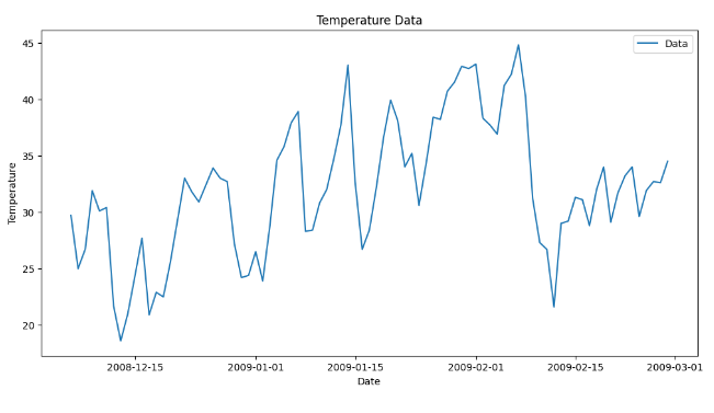
The data is visualized in this step.

Python

# Visualize the data
plt.figure(figsize=(12, 6))
plt.plot( data['Temperature '], label='Data')
plt.xlabel('Date')
plt.ylabel('Temperature')
plt.legend()
plt.title('Temperature Data')
plt.show()

Output:

Step 2: Data Preprocessing

Now that we have our synthetic data, we need to preprocess it. We’ll create lag features, split the data into training and testing sets, and format it for modeling.

• In the first step, the lag features are added to the data frame.
• Then the rows with null values are completely removed.
• The data is then split into training and testing datasets.
• The input features and target variable are defined.

Python3

# Adding lag features to the DataFrame
for i in range(1, 6):  # Creating lag features up to 5 days
    data[f'Lag_{i}'] = data['Temperature '].shift(i)

# Drop rows with NaN values resulting from creating lag features
data.dropna(inplace=True)

# Split the data into training and testing sets
train_size = int(0.8 * len(data))
train_data = data[:train_size]
test_data = data[train_size:]

# Define the input features (lag features) and target variable

y_train = train_data['Temperature ']

y_test = test_data['Temperature ']

ACF Plot

The Autocorrelation Function (ACF) plot is a graphical tool used to visualize and assess the autocorrelation of a time series data at different lags. The ACF plot helps you understand how the current value of a time series is correlated with its past values. You can create an ACF plot in Python using the plot_acf function from the Stats models library.

Python3

from statsmodels.graphics.tsaplots import plot_acf
series = data['Temperature ']
plot_acf(series)
plt.show()

Output:

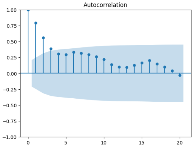
ACF Plot

The graph shows, the autocorrelation values for the first 20 lags. The plot displays autocorrelation values at different lags, with lags on x-axis and autocorrelation values on the y-axis. The graph helps us to identify the significant lags where autocorrelation values are outside the confidence interval (indicated by the shaded region).

We can observe a significant correlation from lag=1 to lag=4. We check the correlation of the lagged values using the approach mentioned below:

Python3

data['Temperature '].corr(data['Temperature '].shift(1))

Output:

0.7997281316018658

Lag=1 provides us with the highest correlation value of 0.799. Similarly, we have checked with lag= 2, 3, 4. For the shift set to 4, we get the correlation as 0.31.

Step 3: Model Building

We’ll build an autoregressive model using AutoReg model.

• We import the required libraries to create the autoregressive model.
• Then we train the autoregressive model on the train data.

Python

from statsmodels.tsa.ar_model import AutoReg
from statsmodels.graphics.tsaplots import plot_acf
from statsmodels.tsa.api import AutoReg
from sklearn.metrics import mean_absolute_error, mean_squared_error

# Create and train the autoregressive model
lag_order = 1 # Adjust this based on the ACF plot
ar_model = AutoReg(y_train, lags=lag_order)
ar_results = ar_model.fit()

Step 4: Model Evaluation

Evaluate the model’s performance using Mean Absolute Error (MAE) and Root Mean Squared Error (RMSE).

• We then make predictions using the AutoReg model and label it as y_pred.
• MAE and RMSE metrics are calculated to evaluate the performance of AutoReg model.

Python

# Make predictions on the test set
y_pred = ar_results.predict(start=len(train_data), end=len(train_data) + len(test_data) - 1, dynamic=False)
#print(y_pred)

# Calculate MAE and RMSE
mae = mean_absolute_error(y_test, y_pred)
rmse = np.sqrt(mean_squared_error(y_test, y_pred))
print(f'Mean Absolute Error: {mae:.2f}')
print(f'Root Mean Squared Error: {rmse:.2f}')

Output:

Mean Absolute Error: 1.59
Root Mean Squared Error: 2.30

In the code, ar_results is an ARIMA model fitted to our time series data. To make predictions on the test set, we use the predict method of the ARIMA model. Here’s how it works:

• start specifies the starting point for prediction. In this case, we start the prediction right after the last data point in our training data, which is equivalent to the first data point in our test set.
• end specifies the ending point for prediction. We set it to the last data point in our test set.
• dynamic=False indicates that we are using out-of-sample forecasting. This means that each forecasted point uses the true values of the previous observations. This is typically used for model evaluation on the test set.
• The predictions are stored in y_pred, which contains the forecasted values for the test set.

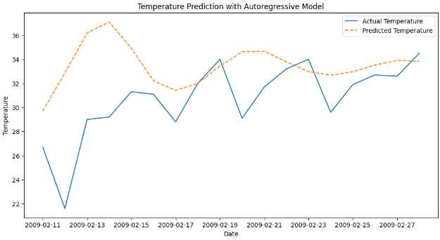
Step 5: Visualization

Visualize the model’s predictions against the actual temperature data. Finally, the predictions made by the AutoReg model are visualized using Matplotlib library.

Actual Predictions Plot:

Python

# Visualize the results
plt.figure(figsize=(12, 6))
plt.plot(test_data["Date"] ,y_test, label='Actual Temperature')
plt.plot( test_data["Date"],y_pred, label='Predicted Temperature', linestyle='--')
plt.xlabel('Date')
plt.ylabel('Temperature')
plt.legend()
plt.title('Temperature Prediction with Autoregressive Model')
plt.show()

Output:

Forecast Plot:

Python

# Define the number of future time steps you want to predict (1 week)
forecast_steps = 7

# Extend the predictions into the future for one year
future_indices = range(len(test_data), len(test_data) + forecast_steps)
future_predictions = ar_results.predict(start=len(train_data), end=len(train_data) + len(test_data) + forecast_steps - 1, dynamic=False)

# Create date indices for the future predictions
future_dates = pd.date_range(start=test_data['Date'].iloc[-1], periods=forecast_steps, freq='D')

# Plot the actual data, existing predictions, and one year of future predictions
plt.figure(figsize=(12, 6))
plt.plot(test_data['Date'], y_test, label='Actual Temperature')
plt.plot(test_data['Date'], y_pred, label='Predicted Temperature', linestyle='--')
plt.plot(future_dates, future_predictions[-forecast_steps:], label='Future Predictions', linestyle='--', color='red')
plt.xlabel('Date')
plt.ylabel('Temperature')
plt.legend()
plt.title('Temperature Prediction with Autoregressive Model')
plt.show()

Output:

Benefits and Drawbacks of Autoregressive Models

Autoregressive models (AR models) are a class of time series models that have their own set of benefits and drawbacks. Understanding these can help in choosing when to use them and when to consider alternative modeling approaches.

Benefits of Autoregressive Models:

• Simplicity: AR models are relatively simple to understand and implement. They rely on past values of the time series to predict future values, making them conceptually straightforward.
• Interpretability: The coefficients in an AR model have clear interpretations. They represent the strength and direction of the relationship between past and future values, making it easier to derive insights from the model.
• Useful for Stationary Data: AR models work well with stationary time series data. Stationary data have stable statistical properties over time, which is an assumption that AR models are built upon.
• Efficiency: AR models can be computationally efficient, especially for short time series or when you have a reasonable amount of data.
• Modeling Temporal Patterns: AR models are good at capturing short-term temporal dependencies and patterns in the data, which makes them valuable for short-term forecasting.

Drawbacks of Autoregressive Models:

• Stationarity Assumption: AR models assume that the time series is stationary, meaning that its statistical properties do not change over time. In practice, many real-world time series are non-stationary, requiring preprocessing steps like differencing.
• Limited to Short-Term Dependencies: AR models are not well-suited for capturing long-term dependencies in data. They are primarily designed for modeling short-term temporal patterns.
• Lag Selection: Choosing the appropriate lag order (p) in an AR model can be challenging. Selecting too few lags may lead to underfitting, while selecting too many may lead to overfitting. Techniques like ACF and PACF plots are used to determine the lag order.
• Sensitivity to Noise: AR models can be sensitive to random noise in the data. This sensitivity can lead to overfitting, especially when dealing with noisy or irregular time series.
• Limited Forecast Horizon: AR models are generally not suitable for long-term forecasting as they are designed for capturing short-term dependencies. For long-term forecasting, other models like ARIMA, SARIMA, or machine learning models may be more appropriate.
• Data Quality Dependence: The effectiveness of AR models is highly dependent on data quality. Outliers, missing values, or data irregularities can significantly affect the model’s performance.

Conclusion

Autoregressive (AR) models provide a powerful framework for analyzing and forecasting time series data. We explored the fundamental concepts of AR models, from understanding autocorrelation to fitting models and making future predictions. By generating a simulated temperature dataset, we were able to apply AR modeling. AR models are particularly useful when dealing with stationary time series data, where past values influence future observations. The choice of lag order is a crucial step, and it can be determined by examining the Autocorrelation Function (ACF) plot.

As we demonstrated, AR models offer a practical approach to forecasting. However, they have their limitations and are most effective when the underlying data exhibits some degree of autocorrelation. For more complex time series data, other models like ARIMA or SARIMA may be more appropriate.

The ability to make accurate forecasts is a valuable asset in various domains, from finance to economics and beyond. By mastering Autoregressive models and understanding their applications, analysts and data scientists can make informed decisions based on historical data, helping to anticipate future trends and make better choices.