Feature Scaling Using R

Feature scaling is a technique to improve the accuracy of machine learning models. This can be done by removing unreliable data points from the training set so that the model can learn useful information about relevant features. Feature scaling is widely used in many fields, including business analytics and clinical data science.

Feature Scaling Using R Programming Language

In R It essentially involves taking an input variable and scaling it down so that its mean value is 0 (or close enough). This will make your model more stable, which can improve its performance – you’ll get better predictions without having to train the model for longer than necessary.

It’s important to note that feature scaling does not come for free: you have to carefully choose which features should be scaled down and when they should be scaled down (and why).

Types of feature scaling

Standardization:

Standardization is the simplest form of scaling, in which all the values are standardized to have a mean of zero and a standard deviation of one. For example, if you had a dataset with two variables (age and height), then you would calculate their means and standard deviations before performing any statistical tests on them.

Feature Scaling Using R

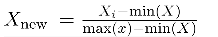
Normalization: 

Normalization method also involves calculating and standardizing every value in your dataset before performing any statistical test but instead finds its median value as well as its mean value. It then determines whether those two values differ significantly from each other based on how far apart they fall from that first reference point; if so then it assumes that there is something wrong with either one or both of them so as not to draw conclusions about what’s happening within our sample population (e.g., “My kid might be taller than average because he grew faster than most kids his age”).

Feature Scaling Using R

Creating a Dataset to apply feature scaling in R

First, we need to create a dataframe.

R

# Age vector
age <- c(19,20,21,22,23,24,24,26,27)

# Salary vector
salary <- c(10000,20000,30000,40000,
            50000,60000,70000,80000,90000)

# Data frame created using age and salary
df <- data.frame( "Age" = age,
                 "Salary" = salary,
                 stringsAsFactors = FALSE)
df

Output:

  Age Salary
1  19  10000
2  20  20000
3  21  30000
4  22  40000
5  23  50000
6  24  60000
7  24  70000
8  26  80000
9  27  90000

Once the dataset is created. Now we can start implementing Feature Scaling.

By using General Formula

We know the formulas for both standardization and normalization. Let’s apply them one by one.

implement standardization

R

data <- data.frame(Age = rnorm(500, 50, 8),
                   Weight = rnorm(500, 80, 10))
data <- as.data.frame(sapply(df, function(x)
                      (x-mean(x))/sd(x)))
data

Output:

          Age     Salary                             
1 -1.45833333 -1.4605935
2 -1.08333333 -1.0954451
3 -0.70833333 -0.7302967
4 -0.33333333 -0.3651484
5  0.04166667  0.0000000
6  0.41666667  0.3651484
7  0.41666667  0.7302967
8  1.16666667  1.0954451
9  1.54166667  1.4605935

implement normalization

R

data2 <- data.frame(Age = rnorm(500, 50, 8),
                   Weight = rnorm(500, 80, 10))
data2 <- as.data.frame(sapply(df, function(x)
                      (x-min(x))/(max(x)-min(x))))
data2

Output:

    Age Salary
1 0.000  0.000
2 0.125  0.125
3 0.250  0.250
4 0.375  0.375
5 0.500  0.500
6 0.625  0.625
7 0.625  0.750
8 0.875  0.875
9 1.000  1.000

Using Caret Library

Let’s import the library caret and then apply the Standardization and Normalisation.

Standardization Using Caret Library

R

# Importing Library
library(caret)

# Standardisation:
data1.pre <- preProcess(df, method=c("center", "scale"))
data1<- predict(data1.pre, df)
data1

Output:

          Age     Salary
1 -1.45833333 -1.4605935
2 -1.08333333 -1.0954451
3 -0.70833333 -0.7302967
4 -0.33333333 -0.3651484
5  0.04166667  0.0000000
6  0.41666667  0.3651484
7  0.41666667  0.7302967
8  1.16666667  1.0954451
9  1.54166667  1.4605935

Normalisation Using Caret Library

R

# Normalisation:
data2.pre <- preProcess(df, method="range")
data2 <- predict(data2.pre, df)
data2

Output:

    Age Salary
1 0.000  0.000
2 0.125  0.125
3 0.250  0.250
4 0.375  0.375
5 0.500  0.500
6 0.625  0.625
7 0.625  0.750
8 0.875  0.875
9 1.000  1.000

Using Dplyr Library

Let’s import the library dplyr and then apply the Standardization and Normalisation.

Standardization Using Dplyr Library

R

# Importing library
library(dplyr)

# Standardization
data2 <- df %>%
mutate_at(vars("Salary"), scale)
data2

Output:

          Age     Salary
1 -1.45833333 -1.4605935
2 -1.08333333 -1.0954451
3 -0.70833333 -0.7302967
4 -0.33333333 -0.3651484
5  0.04166667  0.0000000
6  0.41666667  0.3651484
7  0.41666667  0.7302967
8  1.16666667  1.0954451
9  1.54166667  1.4605935

Normalisation Using Dplyr Library

R

# Importing library
library(dplyr)

# Normalization
data1 <- df %>%
mutate_all(scale)
data1

Output:

  Age     Salary
1  19 -1.4605935
2  20 -1.0954451
3  21 -0.7302967
4  22 -0.3651484
5  23  0.0000000
6  24  0.3651484
7  24  0.7302967
8  26  1.0954451
9  27  1.4605935

Using BBmisc package

BBmisc is an R package so with the help of it we can calculate the standardization and normalization.

Standardization Using BBmisc package

R

# load library
library(BBmisc)

# Normalize the Age and Salary columns using min-max normalization
df_standardized <- BBmisc::normalize(df, method = "standardize")

df_standardized

Output:

           Age     Salary
1 -1.45833333 -1.4605935
2 -1.08333333 -1.0954451
3 -0.70833333 -0.7302967
4 -0.33333333 -0.3651484
5  0.04166667  0.0000000
6  0.41666667  0.3651484
7  0.41666667  0.7302967
8  1.16666667  1.0954451
9  1.54166667  1.4605935

Normalization Using BBmisc package

R

# load library
library(BBmisc)

# Normalize the Age and Salary columns using min-max normalization
df_normalized <- BBmisc::normalize(df, method = "range")

df_normalized

Output:

    Age Salary
1 0.000  0.000
2 0.125  0.125
3 0.250  0.250
4 0.375  0.375
5 0.500  0.500
6 0.625  0.625
7 0.625  0.750
8 0.875  0.875
9 1.000  1.000