Autocorrelation and Partial Autocorrelation

Last Updated : 22 Nov, 2023

Autocorrelation and partial autocorrelation are statistical measures that help analyze the relationship between a time series and its lagged values. In R Programming Language, the acf() and pacf() functions can be used to compute and visualize autocorrelation and partial autocorrelation, respectively.

Autocorrelation

Autocorrelation measures the linear relationship between a time series and its lagged values. In simpler terms, it assesses how much the current value of a series depends on its past values. Autocorrelation is fundamental in time series analysis, helping identify patterns and dependencies within the data.

Mathematical Representation

The autocorrelation function (ACF) at lag k for a time series.

$\rho_k = \frac{\text{Cov}(X_t, X_{t-k})}{\sqrt{\text{Var}(X_t) \cdot \text{Var}(X_{t-k})}}$

Here:

Cov() is the covariance function.
Var() is the variance function.
k is the lag.
$x_t$ is the value of the time series at time t.
$x_{t-k}$ is the value of the time series at time t-k

Interpretation

Positive ACF: A positive ACF at lag k indicates a positive correlation between the current observation and the observation at lag k.
Negative ACF: A negative ACF at lag k indicates a negative correlation between the current observation and the observation at lag k.
Decay in ACF: The decay in autocorrelation as lag increases often signifies the presence of a trend or seasonality in the time series.
Significance: Significant ACF values at certain lags may suggest potential patterns or relationships in the time series.

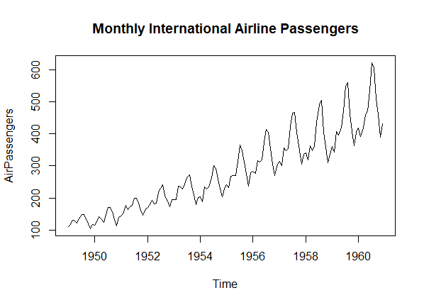
Let’s take an example with a real-world dataset to illustrate the differences between the Autocorrelation Function (ACF) and Partial Autocorrelation Function (PACF). In this example, we’ll use the “AirPassengers” dataset in R, which represents monthly totals of international airline passengers.

R

# Load necessary libraries
library(forecast)
 
# Load AirPassengers dataset
data("AirPassengers")
 
# Plot the time series
plot(AirPassengers, main = "Monthly International Airline Passengers")

Output:

Autocorrelation

Now Plot ACF

R

# Plot ACF
acf(AirPassengers, main = "Autocorrelation Function (ACF) for AirPassengers")

Output:

Autocorrelation

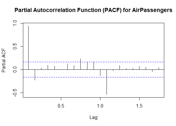
we use the same “AirPassengers” dataset and plot the PACF. The PACF plot shows the direct correlation at each lag, helping identify the order of autoregressive terms.

The ACF plot reveals a decaying pattern, indicating a potential seasonality in the data. Peaks at multiples of 12 (12, 24, …) suggest a yearly cycle, reflecting the seasonal nature of airline passenger data.
The ACF plot gives a comprehensive view of the correlation at all lags, showing how each observation relates to its past values.

Partial Autocorrelation

Partial autocorrelation removes the influence of intermediate lags, providing a clearer picture of the direct relationship between a variable and its past values. Unlike autocorrelation, partial autocorrelation focuses on the direct correlation at each lag.

Mathematical Representation

The partial autocorrelation function (PACF) at lag k for a time series.

$\phi_k = \frac{\text{cov}(X_t, X_{t-k} \mid X_{t-1}, X_{t-2}, \ldots, X_{t-k+1})}{\sqrt{\text{var}(X_t \mid X_{t-1}, X_{t-2}, \ldots, X_{t-k+1}) \cdot \text{var}(X_{t-k} \mid X_{t-1}, X_{t-2}, \ldots, X_{t-k+1})}}$

Here:

$X_t$ is the value of the time series at time.
$X_{t-k}$ : is the value of the time series at time (t-k)
$\text{cov}(X_t, X_{t-k} \mid X_{t-1}, X_{t-2}, \ldots, X_{t-k+1})$ is the conditional covariance between $X_t$ and $X_{t-k}$ given the values of the intermediate lags.
$\text{var}(X_t \mid X_{t-1}, X_{t-2}, \ldots, X_{t-k+1})$ is the conditional variance of $X_t$ given the values of the intermediate lags.
$\text{var}(X_{t-k} \mid X_{t-1}, X_{t-2}, \ldots, X_{t-k+1})$ is the conditional variance of $X_{t-k}$ given the values of the intermediate lags.

Interpretation

Direct Relationship: PACF isolates the direct correlation between the current observation and the observation at lag k, controlling for the influence of lags in between.
AR Process Identification: Peaks or significant values in PACF at specific lags can indicate potential orders for autoregressive (AR) terms in time series models.
Modeling Considerations: Analysts often examine PACF to guide the selection of lag orders in autoregressive integrated moving average (ARIMA) models.

R

# Load necessary libraries
library(forecast)
 
# Load AirPassengers dataset
data("AirPassengers")
 
# Plot PACF
pacf_result <- pacf(AirPassengers, 
                    main = "Partial Autocorrelation Function (PACF) for AirPassengers")

Output:

Partial Autocorrelation

we use the same “AirPassengers” dataset and plot the PACF. The PACF plot shows the direct correlation at each lag, helping identify the order of autoregressive terms.

The PACF plot helps identify the direct correlation at each lag. Peaks at lags 1 and 12 suggest potential autoregressive terms related to the monthly and yearly patterns in the data.
The PACF plot, on the other hand, focuses on the direct correlation at each lag, providing insights into the order of autoregressive terms.
By comparing the two plots, you can observe how they complement each other in revealing the temporal dependencies within the time series. The ACF helps identify overall patterns, while the PACF refines the analysis by highlighting direct correlations.

Perform both on a Time series dataset to compare

R

# Load necessary libraries
library(fpp2)
 
# Load the "ausbeer" dataset from fpp2 package
data("ausbeer")
 
# Plot the time series
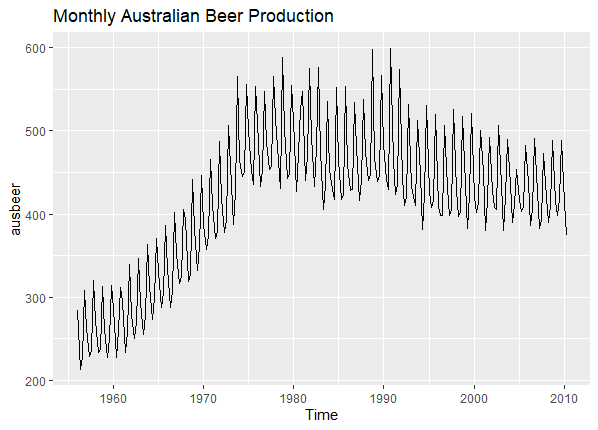
autoplot(ausbeer, main = "Monthly Australian Beer Production")

Output:

Time Series Plot

Plot ACF

R

# Plot ACF
acf(ausbeer, main = "Autocorrelation Function (ACF) for Australian Beer Production")

Output:

Autocorrelation Plot

Plot PACF for differenced time series

R

# Load PACF from the forecast package
library(forecast)
 
# Plot PACF for differenced time series
diff_ausbeer <- diff(ausbeer)
pacf_result <- pacf(diff_ausbeer,main = "Partial Autocorrelation Function (PACF) for
                                  Differenced Australian Beer Production")

Output:

Partial Autocorrelation Plot

In this example, we use the “ausbeer” dataset from the fpp2 package, which represents monthly Australian beer production. The ACF plot can provide insights into the potential seasonality and trends in beer production.

Autocorrelation (ACF): The ACF plot for Australian beer production may reveal patterns related to seasonality, trends, or cyclic behavior. Peaks at certain lags could indicate recurring patterns in beer production.
Partial Autocorrelation (PACF): Differencing the time series and examining the PACF helps identify potential autoregressive terms that capture the direct correlation at each lag, after removing the influence of trends.

Additional Considerations

- Seasonal Differencing: In some cases, it might be beneficial to apply seasonal differencing (e.g., differencing by 12 for monthly data) to handle seasonality properly.
- Seasonal Differencing: In some cases, it might be beneficial to apply seasonal differencing (e.g., differencing by 12 for monthly data) to handle seasonality properly.
- Model Selection: The combination of ACF and PACF analysis can guide the selection of parameters in time series models, such as autoregressive integrated moving average (ARIMA) models.
- Interpretation: Understanding the patterns revealed by ACF and PACF is crucial for interpreting the underlying dynamics of a time series and building accurate forecasting models.

Difference between Autocorrelation and Partial Autocorrelation

Autocorrelation (ACF) and Partial Autocorrelation (PACF) are both measures used in time series analysis to understand the relationships between observations at different time points.

Autocorrelation	Partial Autocorrelation
Used for identifying the order of a moving average (MA) process.	Used for identifying the order of an autoregressive (AR) process.
Represents the overall correlation structure of the time series.	Highlights the direct relationships between observations at specific lags.
Autocorrelation measures the linear relationship between an observation and its previous observations at different lags.	Partial Autocorrelation measures the direct linear relationship between an observation and its previous observations at a specific lag, excluding the contributions from intermediate lags.

Conclusion

ACF and PACF are critical tools in time series analysis, providing insights into temporal dependencies within a dataset. These functions aid in understanding the structure of the data, identifying potential patterns, and guiding the construction of time series models for accurate forecasting. By examining ACF and PACF, analysts gain valuable information about the underlying dynamics of the time series they are studying.

Suggest improvement

How to Calculate Autocorrelation in R?

Share your thoughts in the comments

Autocorrelation and Partial Autocorrelation