Seasonal Decomposition of Time Series by Loess (STL)

Researchers can uncover trends, seasonal patterns, and other temporal linkages by employing time series data, which gathers information across many time-periods. Understanding the underlying patterns and components within time series data is crucial for making informed decisions and predictions. One common challenge in analyzing time series data is dealing with seasonality which is periodic fluctuations that occur at regular intervals. Seasonal patterns can obscure the overall trend and make it challenging to extract meaningful insights from the data. In this article, we will perform seasonal decomposition using Loess(STL) on a time-series dataset and remove the seasonality from the dataset.

What is Time-Series data?

Time series data is a set of observations or measurements taken over repeated, uniformly spaced intervals of time that is commonly used in industries such as finance, economics, climate research, and healthcare. Time series data, as opposed to cross-sectional data, provides insights into how a particular phenomenon evolves, with each data point associated with a specific timestamp, forming a sequence that allows for the analysis of temporal trends and patterns.

What is Seasonal Decomposition?

Seasonal decomposition is a statistical technique for breaking down a time series into its essential components, which often include the trend, seasonal patterns, and residual (or error) components. The goal is to separate the different sources of variation within the data to understand better and analyze each component independently. The fundamental components are discussed below:

• Trend: The underlying long-term progression or direction in the data.
• Seasonal: The repeating patterns or cycles that occur at fixed intervals like daily, monthly or yearly.
• Residual: The random fluctuations or noise in the data that cannot be attributed to the trend or seasonal patterns.

What is Loess (STL)?

Locally Weighted Scatterplot Smoothing or Loess is a non-parametric regression method used for smoothing data. In the context of time series analysis, Seasonal-Trend decomposition using Loess (STL) is a specific decomposition method that employs the Loess technique to separate a time series into its trend, seasonal, and residual components. STL is particularly effective in handling time series data with complex and non-linear patterns. In STL, the decomposition is performed by iteratively applying Loess smoothing to the time series. This process helps capture both short-term and long-term variations in the data, making it a robust method for decomposing time series with irregular or changing patterns.

Why to perform seasonal decomposition?

There are various reasons for performing seasonal decomposition in Time-series data which are discussed below:

1. Pattern Identification: Seasonal decomposition allows analysts to identify and understand the underlying patterns within a time series. This is crucial for recognizing recurring trends, seasonal effects and overall data behavior.
2. Forecasting: Separating a time series into its components facilitates more accurate forecasting. By modeling the trend, seasonal patterns and residuals separately, it becomes possible to make predictions and projections based on the individual components.
3. Anomaly Detection: Detecting anomalies or unusual events in a time series is more effective when the data is decomposed. Anomalies are easier to identify when they stand out against the background of the trend and seasonal patterns.
4. Statistical Analysis: Seasonal decomposition aids in statistical analysis by providing a clearer picture of the structure of the time series. This, in turn, enables the application of various statistical methods and models.

Step-by-step implementation

Importing required modules:

At first, we will import all required Python modules like Pandas, NumPy and Matplotlib etc.

Python3

import pandas as pd
import numpy as np
import matplotlib.pyplot as plt
from statsmodels.tsa.seasonal import STL

Dataset loading and visualization:

Now we will load a simple time-series data and visualize the raw time-series patterns.

Python3

# Load the dataset
url = "https://raw.githubusercontent.com/jbrownlee/Datasets/master/airline-passengers.csv"
df = pd.read_csv(url, parse_dates=['Month'], index_col='Month')

# Plot the original time series
plt.figure(figsize=(7, 4))
plt.plot(df.index, df['Passengers'], label='Original Time Series', color='green')
plt.title('Air Passengers Dataset')
plt.xlabel('Year')
plt.ylabel('Number of Passengers')
plt.legend()
plt.show()

Output:

Raw data visualization

The above plot is the raw time-series of the dataset where we have plotted the ‘Year’ to the X-axis and ‘Number of Passengers’ to the Y-axis. From this plot we can see the there is a presence of similar pattern or seasonal component which is being repeated with the forward of X-axis which is ‘Year’ or time-interval. Now in the next step we will perform decomposition.

Decomposition using Loess(STL)

Now we will perform STL decomposition on the time-series data and to do this we need to specify some hyper-parameters which are listed below:

1. seasonal: This parameter defines the periodicity of the seasonal component. In our code, we will set it to 13 which suggests a seasonal period of 13 time points. This is suitable for monthly data where we might expect a yearly seasonality (12 months) plus some additional flexibility. Remember that, the value seasonal should be odd number (default is 7).
2. robust: This parameter is a Boolean flag that determines whether to use robust estimation in the Loess smoothing step. When set to ‘True', robust smoothing is applied, meaning the method will be less sensitive to outliers in the data. This can be beneficial when dealing with time series that may have irregularities or extreme values.

Python3

# Perform STL decomposition
stl = STL(df['Passengers'], seasonal=13, robust=True)
result = stl.fit()

# Plot the decomposition components
fig, (ax1, ax2, ax3) = plt.subplots(3, 1, figsize=(7, 4))

ax1.plot(df.index, result.trend, label='Trend', color='red')
ax1.set_title('Trend Component')
ax2.plot(df.index, result.seasonal, label='Seasonal', color='blue')
ax2.set_title('Seasonal Component')
ax3.plot(df.index, result.resid, label='Residual')
ax3.set_title('Residual Component')
plt.tight_layout()
plt.show()

Output:

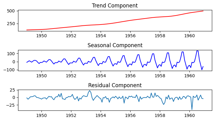
Components of Time-series data after decomposition

The above plot consists of all time-series components which are trend, seasonal and residual. As we have already seen in raw dataset plot that the seasonal component is repeated with higher magnitude when we go forward with X-axis. Here also, we can visualize that the seasonal component is increasing gradually with time. However, the trend component is very straight forward without any sudden change and residual component presents that the dataset has noises but not high yet.

Removing seasonal component

Now we will remove the seasonal component from the actual time-series data. This will make the data suitable for any further implementations like forecasting etc.

Python3

# Create a deseasonalized time series
deseasonalized_series = df['Passengers'] - result.seasonal

# visualize the comparative plot
plt.figure(figsize=(7, 4))
plt.plot(df.index, df['Passengers'], label='Original Time Series', color='blue')
plt.plot(df.index, deseasonalized_series, label='Deseasonalized Time Series', color='green')
plt.title('Original vs. Deseasonalized Time Series')
plt.xlabel('Year')
plt.ylabel('Number of Passengers')
plt.legend()
plt.show()

Output:

Comparative plot

The above plot is the comparative plot between original and de-seasonalized time-series which correctly shows that how easy and simple the data looks like when we remove the seasonal component. Now this de-seasonalized data can be useful for various further complex tasks like forecasting and recommendation system where model training is required. It is always suggested to perform seasonal decomposition and removal in time-series data to make it accurate for model predictions.

Conclusion

We can conclude that, seasonal decomposition of any Time-series data is very essential for application based forecasting or recommendation system as seasonality can induce unexpected errors in the results. Loess (STL) is an effective technique to decompose time-series data and make it smooth and normalized.