Multivariate Time Series Forecasting with LSTMs in Keras

Multivariate forecasting entails utilizing multiple time-dependent variables to generate predictions. This forecasting approach incorporates historical data while accounting for the interdependencies among the variables within the model. In this article, we will explore the world of multivariate forecasting using LSTMs, peeling back the layers to understand its core, explore its applications, and grasp the revolutionary influence it has on steering decision-making towards the future.

What is Multivariate forecasting?

Multivariate Forecasting is a statistical technique to employ future values for multiple interconnected variables simultaneously. The process of multivariate forecasting begins by collecting historical data for all the features and then these datasets are analyzed to identify patterns, correlations based on relationships, and predict the future values.

Common techniques utilized in multivariate forecasting include Vector Autoregression (VAR), which models the interdependencies between multiple time series variables, and structural equation modeling (SEM), which allows for the examination of complex relationships between variables. Moreover, machine learning algorithms like neural networks and gradient boosting machines have also been increasingly employed in multivariate forecasting tasks due to their ability to capture intricate patterns and nonlinear relationships within data.

What is LSTM?

Long-term short-term memory represents a major advancement of recurrent neural networks (RNNs) in Deep Learning. This sophisticated algorithm solves and achieve challenges associated with moderate extinction high praise for his exceptional skill in sequencing data in natural language processing, speech recognition etc. Provides the ability to excel in a variety of applications. Essentially, LSTMs act as intelligent information processors, which can be identified when they are trusted which are subtle and offer unmatched performance in projects where a detailed understanding of temporal relationships is paramount.

Key points of Multivariate forecasting using LSTM

Some of the key-points of Multivariate forecasting using LSTM is discussed below:

1. Multivariate Marvels: Multivariate time series forecasting is all about predicting not just one but multiple variables over time, offering a holistic view of data dynamics.
2. Forecast with details: Imagine a stock price forecast that goes beyond only Closing price predictions – it includes Opening prices, Daily highest pick, Daily Lowest prices etc. Multivariate forecasting brings this level of detail to our data predictions.
3. LSTM Superstars: Enter into Long Short-Term Memory (LSTM) networks, the rockstars of neural networks. Unlike regular algorithms, LSTMs come equipped with memory powers, allowing them to capture intricate relationships in our data, making them perfect for unraveling complex multivariate patterns.
4. Coding Magic with Keras: Keras, the wizard’s wand of the coding world, steps in to make working with LSTMs a breeze. It transforms the complex into the manageable, and even injects a bit of enjoyment and time-efficiency into the coding sorcery.

Step-by-step implementation of Multivariate Forecast using LSTM

Importing required modules

For the implementation, we are going to import datatime module, sklearn, numpy, pandas, math, keras, matplotlib.pyplot and TensorFlow.

Python3

import datetime
import sklearn
from sklearn.impute import SimpleImputer
from sklearn.preprocessing import MinMaxScaler
from sklearn.decomposition import KernelPCA
import numpy as np
import pandas as pd
import math
import keras
import matplotlib.pyplot as plt
import tensorflow as tf
tf.random.set_seed(99)

Dataset loading

Now, we will load a time-series dataset.

Python3

# Dataset loading
dataFrame = pd.read_csv('final_data_adj.csv')  # https://github.com/SusmitSekharBhakta/Stock-market-price-prediction/blob/main/final_data_adj.csv

Data preprocessing

Using the following code, we will preprocess the data by handling missing values, dropping irrelevant columns, scaling features, and scaling target variables, preparing it for the further analysis or modeling.

Python3

imputer = SimpleImputer(missing_values=np.nan)  # Handling missing values
dataFrame.drop(columns=['Date'], inplace=True)
dataFrame = pd.DataFrame(imputer.fit_transform(dataFrame), columns=dataFrame.columns)
dataFrame = dataFrame.reset_index(drop=True)
# Applying feature scaling
scaler = MinMaxScaler(feature_range=(0, 1))
df_scaled = scaler.fit_transform(dataFrame.to_numpy())
df_scaled = pd.DataFrame(df_scaled, columns=list(dataFrame.columns))
target_scaler = MinMaxScaler(feature_range=(0, 1))
df_scaled[['Open', 'Close']] = target_scaler.fit_transform(dataFrame[['Open', 'Close']].to_numpy())
df_scaled = df_scaled.astype(float)

Data preparation

A function called singleStepSampler is introduced to facilitate the preparation of the dataset for single-step time-series forecasting.

This function takes two parameters: a dataframe, denoted as df, and a specified window size. Within the function, two lists, namely xRes and yRes, are initialized to serve as containers for input features and target values, respectively. The function utilizes two nested loops to iterate over the rows of the dataframe, creating sequences of input features (xRes) and corresponding target values (yRes) based on the provided window size. The input features are structured as a sequence of windowed data points, where each data point is a list containing values from every column of the dataframe. Target values, sourced from the ‘Open’ and ‘Close’ columns for each window, are appended to yRes.

Ultimately, the function returns numpy arrays xRes and yRes, encapsulating the prepared input features and target values for subsequent time-series forecasting.

Python3

# Single step dataset preparation
def singleStepSampler(df, window):
    xRes = []
    yRes = []
    for i in range(0, len(df) - window):
        res = []
        for j in range(0, window):
            r = []
            for col in df.columns:
                r.append(df[col][i + j])
            res.append(r)
        xRes.append(res)
        yRes.append(df[['Open', 'Close']].iloc[i + window].values)
    return np.array(xRes), np.array(yRes)

Data Splitting

Now we will split the dataset in training and testing sets in 85:15 ratio.

Python3

# Dataset splitting
SPLIT = 0.85
(xVal, yVal) = singleStepSampler(df_scaled, 20)
X_train = xVal[:int(SPLIT * len(xVal))]
y_train = yVal[:int(SPLIT * len(yVal))]
X_test = xVal[int(SPLIT * len(xVal)):]
y_test = yVal[int(SPLIT * len(yVal)):]

Defining LSTM model

In this stage, a multivariate Long Short-Term Memory neural network model is crafted using TensorFlow’s Keras API. The model is initialized as a sequential model, representing a linear stack of layers. The architecture encompasses an LSTM layer with 200 units, designed to process input sequences with a shape defined by the number of features (columns) in the training data (X_train). To prevent overfitting, a dropout layer is introduced. The output layer is a dense layer with 2 units, aligning with the predicted values for the two predictor variables (‘Open’ and ‘Close’). The activation function for this output layer is set to linear. For training, the model is compiled utilizing mean squared error as the loss function, with Mean Absolute Error (MAE) as metrics for further evaluation. The Adam optimizer is employed to facilitate the training process. The summary() method provides a comprehensive overview of the model’s architecture, detailing the number of parameters and layer configurations for enhanced understanding.

Python3

multivariate_lstm = keras.Sequential()
multivariate_lstm.add(keras.layers.LSTM(200, input_shape=(X_train.shape[1], X_train.shape[2])))
multivariate_lstm.add(keras.layers.Dropout(0.2))
multivariate_lstm.add(keras.layers.Dense(2, activation='linear'))
multivariate_lstm.compile(loss = 'MeanSquaredError', metrics=['MAE'], optimizer='Adam')
multivariate_lstm.summary()

Output:

Model: "sequential"
_________________________________________________________________
 Layer (type)                Output Shape              Param #   
=================================================================
 lstm (LSTM)                 (None, 200)               172800    
                                                                 
 dropout (Dropout)           (None, 200)               0         
                                                                 
 dense (Dense)               (None, 2)                 402       
                                                                 
=================================================================
Total params: 173202 (676.57 KB)
Trainable params: 173202 (676.57 KB)
Non-trainable params: 0 (0.00 Byte)
_________________________________________________________________

Model training

Now ,we will train our model on 20 epochs.

Python3

history = multivariate_lstm.fit(X_train, y_train, epochs=20)

Output:

Epoch 1/20
48/48 [==============================] - 6s 8ms/step - loss: 0.0187 - MAE: 0.0877
Epoch 2/20
48/48 [==============================] - 1s 12ms/step - loss: 0.0023 - MAE: 0.0363
Epoch 3/20
48/48 [==============================] - 0s 9ms/step - loss: 0.0019 - MAE: 0.0330
Epoch 4/20
48/48 [==============================] - 0s 8ms/step - loss: 0.0014 - MAE: 0.0289
Epoch 5/20
48/48 [==============================] - 0s 5ms/step - loss: 0.0014 - MAE: 0.0282
Epoch 6/20
48/48 [==============================] - 0s 5ms/step - loss: 0.0013 - MAE: 0.0275
Epoch 7/20
48/48 [==============================] - 0s 5ms/step - loss: 0.0011 - MAE: 0.0258
Epoch 8/20
48/48 [==============================] - 0s 5ms/step - loss: 0.0011 - MAE: 0.0252
Epoch 9/20
48/48 [==============================] - 0s 5ms/step - loss: 0.0011 - MAE: 0.0249
Epoch 10/20
48/48 [==============================] - 0s 5ms/step - loss: 0.0010 - MAE: 0.0241

Forecasting

This code segment focuses on visualizing the multivariate time-series forecasting results using an LSTM model. Initially, the dataset is reloaded with the ‘Date’ column serving as the index. The ‘Date’ column is converted to a datetime format, and the index is set accordingly. The LSTM model (`multivariate_lstm`) is employed to predict values for the test set (`X_test`). The predictions, along with the actual values (`y_test`), are organized into a DataFrame (`d`). The correct date index is assigned to this DataFrame, aligning it with the original dataset. Subsequently, a plot is created using Matplotlib to showcase the actual and predicted values over time. The actual values for ‘Open’ and ‘Close’ are plotted, while the predicted values are represented with dashed lines. Additionally, a portion of the plot is highlighted in a different color, denoted as ‘lightgreen’, corresponding to the forecasted period. This visual distinction aids in easily identifying the forecasted portion within the overall plot. The resulting plot provides a clear representation of the model’s performance, allowing for a visual comparison between predicted and actual values, and highlighting the forecasted period for further analysis.

Python3

# Reload the data with the date index
dataFrame = pd.read_csv('/content/final_data_adj.csv')  # Assuming the CSV file contains a 'Date' column
dataFrame['Date'] = pd.to_datetime(dataFrame['Date'])
dataFrame.set_index('Date', inplace=True)

# Forecast Plot with Dates on X-axis
predicted_values = multivariate_lstm.predict(X_test)

d = {
    'Predicted_Open': predicted_values[:, 0],
    'Predicted_Close': predicted_values[:, 1],
    'Actual_Open': y_test[:, 0],
    'Actual_Close': y_test[:, 1],
}

d = pd.DataFrame(d)
d.index = dataFrame.index[-len(y_test):]  # Assigning the correct date index

fig, ax = plt.subplots(figsize=(10, 6))
#  highlight the  forecast
highlight_start = int(len(d) * 0.9)
highlight_end = len(d) - 1  # Adjusted to stay within bounds
# Plot the actual values
plt.plot(d[['Actual_Open', 'Actual_Close']][:highlight_start], label=['Actual_Open', 'Actual_Close'])

# Plot predicted values with a dashed line
plt.plot(d[['Predicted_Open', 'Predicted_Close']], label=['Predicted_Open', 'Predicted_Close'], linestyle='--')

# Highlight the forecasted portion with a different color
plt.axvspan(d.index[highlight_start], d.index[highlight_end], facecolor='lightgreen', alpha=0.5, label='Forecast')

plt.title('Multivariate Time-Series forecasting using LSTM')
plt.xlabel('Dates')
plt.ylabel('Values')
ax.legend()
plt.show()

Output:

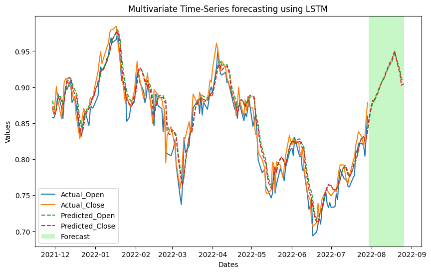
Actual vs. Predicted and future price forecast

Model evaluation

Now we will evaluate the model’s performance in terms of MSE, MAE and R2-Score for each predictor variable.

Python3

# Model Evaluation
def eval(model):
    return {
        'MSE': sklearn.metrics.mean_squared_error(d[f'Actual_{model.split("_")[1]}'].to_numpy(), d[model].to_numpy()),
        'MAE': sklearn.metrics.mean_absolute_error(d[f'Actual_{model.split("_")[1]}'].to_numpy(), d[model].to_numpy()),
        'R2': sklearn.metrics.r2_score(d[f'Actual_{model.split("_")[1]}'].to_numpy(), d[model].to_numpy())
    }

result = dict()

for item in ['Predicted_Open', 'Predicted_Close']:
    result[item] = eval(item)

result

Output:

{'Predicted_Open': {'MSE': 0.0003399016874267341,
  'MAE': 0.014677578549558692,
  'R2': 0.9175119938700349},
 'Predicted_Close': {'MSE': 0.0007753355953061959,
  'MAE': 0.02312380270519607,
  'R2': 0.8091037332332098}}

In conclusion, we can see that for both the predictor variables the errors are very less and R2-score is high enough. It depicts that our LSTM model is performing very well but can perform better with hyper-parameter tuning and advance loss reduction.