Seasonality Detection in Time Series Data

Time series analysis is a fundamental area of study in statistics and data science that provides a powerful framework for understanding and predicting patterns in sequential data. Time series data, in particular, captures information over successive intervals of time, which allows analysts to uncover trends, seasonal patterns, and other temporal dependencies. Among the various aspects of time series analysis, the detection of seasonality plays a crucial role in revealing recurring patterns within the data. In this article, we will detect seasonality in time-series data and remove it from the data, which will make the time-series data more suitable for model training.

What is time series data?

Time series data is a collection of observations or measurements recorded over successive, equally spaced intervals of time which is prevalent in various fields like finance, economics, climate science, and healthcare. Unlike cross-sectional data which captures observations at a single point in time, time series data provides insights into how a particular phenomenon evolves over time where each data point is associated with a specific timestamp, forming a sequence which allows for the analysis of temporal trends and patterns.

What is seasonality?

Seasonality refers to the recurring and predictable patterns that occur at regular intervals within a time series. These patterns often follow a cyclic or periodic nature and can be influenced by various factors like weather, holidays, or business cycles. In the context of time series analysis, seasonality manifests as periodic fluctuations that repeat over fixed time intervals like days, months, or years. Identifying seasonality is crucial for understanding the inherent structure of the data and can aid in making informed decisions, particularly in forecasting and planning.

Why to Detect Seasonality in Time Series Data?

There are some specific reasons which are discussed below:

1. Pattern Recognition: Seasonality detection allows analysts to recognize and understand recurring patterns within a time series which is valuable for interpreting historical trends and making informed predictions about future behavior.
2. Forecasting: Seasonal components significantly impact forecasting accuracy. By detecting seasonality, analysts can account for these patterns when building predictive models which leads to more robust and reliable forecasts.
3. Anomaly Detection: Seasonality detection can help identify anomalies or irregularities in the data. Sudden deviations from the expected seasonal pattern may signal important events or changes that warrant further investigation.
4. Optimized Decision-Making: Understanding seasonality enables organizations to optimize resource allocation, inventory management and marketing strategies based on anticipated temporal fluctuations in demand or other relevant metrics.

Step-by-step implementation

Importing required modules

At first, we will import all required Python modules like Pandas, NumPy, Matplotlib and Seaborn etc.

Python3

import pandas as pd
import numpy as np
import matplotlib.pyplot as plt
import seaborn as sns
from statsmodels.tsa.seasonal import seasonal_decompose

Dataset loading and visualization

Now we will load a time-series dataset from Kaggle. Then we will visualize the raw data.

Python3

# Load the dataset
data = pd.read_csv('AirPassengers.csv')
data['Month'] = pd.to_datetime(data['Month'], format='%Y-%m')
data.set_index('Month', inplace=True)

# Plot the original time series data
plt.figure(figsize=(7, 5))
plt.plot(data, label='Original Time Series')
plt.title('Air Passengers Time Series')
plt.xlabel('Year')
plt.ylabel('Number of Passengers')
plt.legend()
plt.show()

Output:

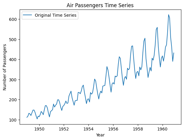
The time-series plot of the dataset

Data decomposition

As we have already got the time-series plot, now we will decompose it to the trend, seasonal and residual components. To do this we need to specify some of the parameters of seasonal decompose function which are listed below–>

• data: This parameter represents the time series data that we want to decompose which is should be in a pandas Data Frame or Series with a datetime index.
• model: This parameter specifies the type of decomposition to be performed which can take two values ‘additive’ or ‘multiplicative’. Here we will use ‘multiplicative’ model as we can see the amplitude of seasonal component is relatively constant(means the pattern is constant) across different levels of the time series. In a multiplicative model, the seasonal and trend components are multiplied rather than added(Additive model).
• extrapolate_trend: This parameter controls whether to extrapolate the trend component to cover missing values at the end of the time series. Here we will set it to 'freq' means that the trend component is extrapolated using the frequency of the time series. Extrapolating the trend can be useful when there are missing values at the end of the time series.

Python3

# Decompose the time series into trend, seasonal and residual components
result = seasonal_decompose(data, model='multiplicative', extrapolate_trend='freq')
result.plot()
plt.suptitle('Seasonal Decomposition of Air Passengers Time Series')
plt.tight_layout()
plt.show()

Output:

Seasonal, Trend and Residue components of the data

Visualizing the seasonality

Now we will visualize the only seasonal component by extracting it from the decomposition results.

Python3

# Plot the seasonal component
plt.figure(figsize=(6, 4))
plt.plot(result.seasonal, label='Seasonal Component')
plt.title('Seasonal Component of Air Passengers Time Series')
plt.xlabel('Year')
plt.ylabel('Seasonal Component')
plt.legend()
plt.show()

Output:

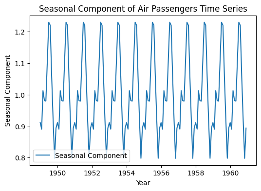
The seasonality of the time-series data

Removing seasonality from the data

To use a time-series data for various purposes including model training it is required to have a seasonality free time-series data. Here we will visualize how organized it will look after removing the seasonality.

Python3

# Plotting the original data and original data without the seasonal component
plt.figure(figsize=(7, 4))
# Plot the original time series data
plt.plot(data, label='Original Time Series', color='blue')
data_without_seasonal = data['#Passengers'] / result.seasonal
# Plot the original data without the seasonal component
plt.plot(data_without_seasonal, label='Original Data without Seasonal Component', color='green')
plt.title('Air Passengers Time Series with and without Seasonal Component')
plt.xlabel('Year')
plt.ylabel('Number of Passengers')
plt.legend()
plt.show()

Output:

Original data vs. seasonality removed data

From the plot we can see that after removing seasonality the time-series data became very organized which required for model training for any further purposes.

Conclusion

We can conclude that seasonality detection and remove it from the data is very important step before proceed to the model training phase. Seasonality can degrade the performance of the predictive model which may lead to wrong forecast.