Understanding Partial Autocorrelation Functions (PACF) in Time Series Data

Partial autocorrelation functions (PACF) play a pivotal role in time series analysis, offering crucial insights into the relationship between variables while mitigating confounding influences. In essence, PACF elucidates the direct correlation between a variable and its lagged values after removing the effects of intermediary time steps. This statistical tool holds significance across various disciplines, including economics, finance, meteorology, and more, enabling analysts to unveil hidden patterns and forecast future trends with enhanced accuracy.

What is Partial Autocorrelation?

Partial correlation is a statistical method used to measure how strongly two variables are related while considering and adjusting for the influence of one or more additional variables. In more straightforward terms, it helps assess the connection between two variables by factoring in the impact of other relevant variables, providing a more nuanced understanding of their relationship.

The correlation between two variables indicates how much they change together. Nonetheless, partial correlation takes an additional step by considering the potential influence of other variables that might be affecting this relationship. In this way, partial correlation seeks to unveil the distinctive connection between two variables by eliminating the shared variability with the control variables.

In terms of mathematical expression, the partial correlation coefficient which assesses the relationship between variables X and Y while considering the influence of variable Z, is typically calculated using the given formula:

Here,

• is the correlation coefficient between X and Y.
• is the correlation coefficient between X and Z.
• is the correlation coefficient between Y and Z.

The numerator represents the correlation between X and Y after accounting for their relationships with Z. The denominator normalizes the correlation by removing the effects of Z.

What are Partial Autocorrelation Functions?

In the realm of time series analysis, the Partial Autocorrelation Function (PACF) measures the partial correlation between a stationary time series and its own past values, considering and accounting for the values at all shorter lags. This is distinct from the Autocorrelation Function, which doesn’t factor in the influence of other lags.

The PACF is a crucial tool in data analysis, particularly for identifying the optimal lag in an autoregressive (AR) model. It became integral to the Box–Jenkins approach to time series modeling. By examining the plots of partial autocorrelation functions, analysts can determine the appropriate lags (often denoted as p) in an AR(p) model or an extended ARIMA(p,d,q) model. This helps in understanding and capturing the temporal dependencies in the data, aiding in effective time series modeling and forecasting.

Calculation of PACF

The Durbin–Levinson Algorithm is employed to compute the theoretical partial autocorrelation function of a stationary time series.

here,

• is the partial autocorrelation at lag k.
• is the autocovariance at lag k.
• represents the partial autocorrelation at lag i, where i ranges from 1 to k-1.

The provided formula can be utilized by incorporating sample autocorrelations to determine the sample partial autocorrelation function for a given time series.

Interpretation of PACF

• Peaks or troughs in the PACF indicate significant lags where there is a strong correlation between the current observation and that specific lag. Each peak represents a potential autoregressive term in the time series model.
• The point at which the PACF values drop to insignificance (i.e., within the confidence interval) suggests the end of the significant lags. The cut-off lag helps determine the order of the autoregressive process.
• If there is a significant peak at lag “p” in the PACF and the values at subsequent lags drop to insignificance, it suggests an autoregressive process of order p(AR(p)) is appropriate for modeling the time series.

Difference Between ACF and PACF

Autocorrelation Function (ACF)	Partial Autocorrelation Function (PACF)
ACF measures the correlation between a data point and its lagged values, considering all intermediate lags. It gives a broad picture of how each observation is related to its past values.	PACF isolates the direct correlation between a data point and a specific lag, while controlling for the influence of other lags. It provides a more focused view of the relationship between a data point and its immediate past.
ACF does not isolate the direct correlation between a data point and a specific lag. Instead, it includes the cumulative effect of all intermediate lags.	PACF is particularly useful in determining the order of an autoregressive (AR) process in time series modeling. Significant peaks in PACF suggest the number of lag terms needed in an AR model.
ACF is helpful in identifying repeating patterns or seasonality in the data by examining the periodicity of significant peaks in the correlation values.	The point where PACF values drop to insignificance helps identify the cut-off lag, indicating the end of significant lags for an AR process.

Partial Autocorrelation Functions using Python

Using Custom Generated dataset

Let’s compute the Partial Autocorrelation Function (PACF) using statsmodels library in Python.

Importing Libraries:

Python3

import pandas as pd
import numpy as np
from statsmodels.tsa.stattools import pacf
from statsmodels.graphics.tsaplots import plot_pacf

• pandas as pd: Imports the Pandas library with an alias pd. Pandas is commonly used for handling structured data.
• numpy as np: Imports the NumPy library with an alias np. NumPy is used for numerical computations.
• from statsmodels.tsa.stattools import pacf: Imports the pacf function from the statsmodels library. This function is used to compute the Partial Autocorrelation Function (PACF) values.

Generating Time Series Data:

Python3

np.random.seed(42)
time_steps = np.linspace(0, 10, 100)
data = np.sin(time_steps) + np.random.normal(scale=0.2, size=len(time_steps))

• np.random.seed(42): Sets the seed for random number generation in NumPy to ensure reproducibility.
• time_steps = np.linspace(0, 10, 100): Creates an array of 100 evenly spaced numbers from 0 to 10.
• data = np.sin(time_steps) + np.random.normal(scale=0.2, size=len(time_steps)): Generates a sine wave using np.sin(time_steps) and adds random noise using np.random.normal() to create a synthetic time series data. This data mimics a sine wave pattern with added noise.

Computing and Plotting PACF :

• pacf_values = pacf(data, nlags=20): Calculates the Partial Autocorrelation Function (PACF) values using the pacf function from statsmodels. It computes PACF values for the provided data with a specified number of lags (nlags=20). Change nlags according to the length of your time series data or the number of lags you want to investigate.
• PACF Plotting: Create a plot representing the PACF values against lags to visualize partial correlations. Set title, labels for axes, and display the PACF plot.
• for lag, pacf_val in enumerate(pacf_values): Iterates through the computed PACF values. The enumerate() function provides both the lag number (lag) and the corresponding PACF value (pacf_val), which are then printed for each lag.

Python3

pacf_values = pacf(data, nlags=20)

# Print PACF values
print("Partial Autocorrelation Function (PACF) values:")
for lag, pacf_val in enumerate(pacf_values):
    print(f"Lag {lag}: {pacf_val}")


# Plot PACF
plt.figure(figsize=(10, 5))
plot_pacf(data, lags=20)  # Change lags according to your data
plt.title('Partial Autocorrelation Function (PACF)')
plt.xlabel('Lags')
plt.ylabel('PACF')
plt.grid(True)
plt.show()

Output:

Partial Autocorrelation Function (PACF) values:
Lag 0: 1.0
Lag 1: 0.9277779190634952
Lag 2: 0.39269022809503606
Lag 3: 0.15463548623480705
Lag 4: -0.03886302489844257
Lag 5: -0.042933753723446405
Lag 6: -0.3632570559137871
Lag 7: -0.2817338901669104
Lag 8: -0.3931692351265865
Lag 9: -0.16550939301708287
Lag 10: -0.27973978478073214
Lag 11: 0.1370484695314932
Lag 12: -0.20445377972909687
Lag 13: -0.12087299096297043
Lag 14: 0.046229571707022764
Lag 15: -0.3654906423192799
Lag 16: -0.36058859364402557
Lag 17: -0.4949891744857339
Lag 18: -0.3466588099640611
Lag 19: -0.30607850279663795
Lag 20: -0.3277911710431029

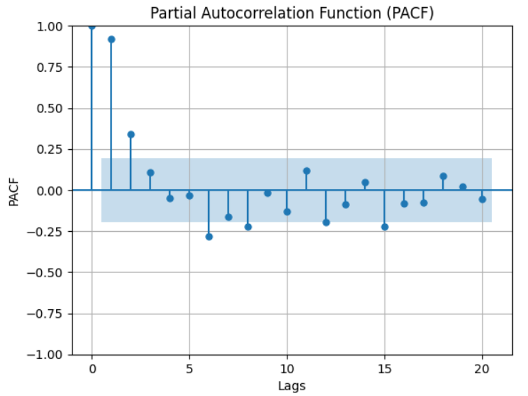
These values represent the Partial Autocorrelation Function (PACF) values calculated for each lag.

Each line in the output indicates the lag number and its corresponding PACF value. Positive or negative values indicate positive or negative correlations respectively, while values close to zero suggest weaker correlations at that lag.

Using Real world Dataset

Importing Required Libraries and Dataset Retrieval

• Imports: Import necessary libraries such as Pandas for data manipulation, Matplotlib for plotting, pacf from statsmodels.tsa.stattools for PACF computation, and get_rdataset from statsmodels.datasets to obtain the ‘AirPassengers’ dataset.
• Loading Dataset: Retrieve the ‘AirPassengers’ dataset using get_rdataset. Convert the index to datetime format.

Python3

import pandas as pd
import matplotlib.pyplot as plt
from statsmodels.tsa.stattools import pacf
from statsmodels.datasets import get_rdataset

# Load the 'AirPassengers' dataset from statsmodels
data = get_rdataset('AirPassengers').data

# Convert the index to datetime format
data.index = pd.to_datetime(data['time'])

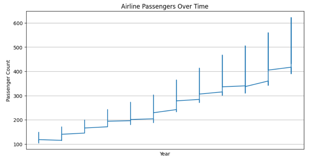
Plotting Time Series Data

• Time Series Plotting: Create a figure and plot the ‘AirPassengers’ time series data using Matplotlib. Set title, labels for axes, and display the plot.

Python3

# Plot the time series data
plt.figure(figsize=(10, 5))
plt.plot(data['value'])
plt.title('Airline Passengers Over Time')
plt.xlabel('Year')
plt.ylabel('Passenger Count')
plt.grid(True)
plt.show()

Output:

Calculating and Plotting PACF

• PACF Computation: Compute the Partial Autocorrelation Function (PACF) values for the ‘AirPassengers’ dataset using pacf from statsmodels. Define the number of lags as 20.
• PACF Plotting: Create a bar plot representing the PACF values against lags to visualize partial correlations. Set title, labels for axes, and display the PACF plot.

Python3

# Calculate PACF using statsmodels pacf function
pacf_values = pacf(data['value'], nlags=20)

# Plot PACF
plt.figure(figsize=(10, 5))
plt.bar(range(len(pacf_values)), pacf_values)
plt.title('Partial Autocorrelation Function (PACF)')
plt.xlabel('Lags')
plt.ylabel('PACF')
plt.grid(True)
plt.show()

Output:

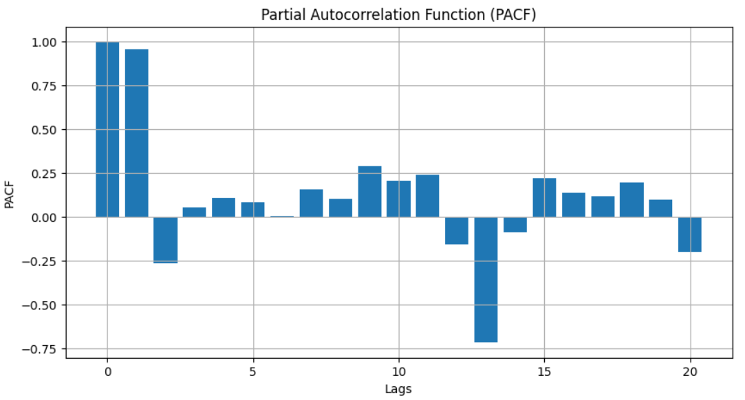
Interpreting PACF plots involves identifying these significant spikes or “partial correlations.” A significant spike at a particular lag implies a strong correlation between the variable and its value at that lag, independent of the other lags. For instance, a PACF plot showcasing a significant spike at lag 1 but no significant spikes at subsequent lags suggests a first-order autoregressive process, often denoted as AR(1) in time series analysis.

Applications in Time Series Analysis

The application of PACF extends to various aspects of time series analysis:

1. Model Identification: PACF aids in identifying the order of autoregressive terms in autoregressive integrated moving average (ARIMA) models. The distinct spikes in the PACF plot indicate the number of autoregressive terms required to model the data accurately.
2. Feature Selection: In predictive modeling, especially in forecasting tasks, understanding the significant lags through PACF helps select relevant features that contribute meaningfully to the predictive power of the model.
3. Diagnostic Checks: PACF plots are indispensable for diagnosing residual autocorrelation in time series models. Deviations from expected PACF patterns can signify model inadequacies or errors.

Limitations and Considerations

While PACF is a powerful tool, it does have certain limitations. It assumes linearity and stationarity in the data, which might not hold true for all-time series. Moreover, interpreting PACF plots might be challenging in cases of noisy or complex data, requiring supplementary analyses or adjustments.

Conclusion

In the realm of time series analysis, partial autocorrelation functions stand as a fundamental tool, enabling analysts to disentangle complex relationships between variables and their lagged values. By revealing direct correlations while mitigating confounding factors, PACF aids in model development, forecasting, and diagnostic evaluations. As data analysis methodologies evolve, the role of PACF remains pivotal, facilitating deeper insights and more accurate predictions in diverse fields where time series data is paramount.