Regression and its Types in R Programming
Last Updated :
29 Nov, 2021
Regression analysis is a statistical tool to estimate the relationship between two or more variables. There is always one response variable and one or more predictor variables. Regression analysis is widely used to fit the data accordingly and further, predicting the data for forecasting. It helps businesses and organizations to learn about the behavior of their product in the market using the dependent/response variable and independent/predictor variable. In this article, let us learn about different types of regression in R programming with the help of examples.
Types of Regression in R
There are mainly three types of Regression in R programming that is widely used. They are:
Linear Regression
The Linear Regression model is one of the widely used among three of the regression types. In linear regression, the relationship is estimated between two variables i.e., one response variable and one predictor variable. Linear regression produces a straight line on the graph. Mathematically
where,
- x indicates predictor or independent variable
- y indicates response or dependent variable
- a and b are coefficients
Implementation in R
In R programming, lm() function is used to create linear regression model.
Syntax: lm(formula)
Parameter:
formula: represents the formula on which data has to be fitted To know about more optional parameters, use below command in console: help(“lm”)
Example: In this example, let us plot the linear regression line on the graph and predict the weight-based using height.
R
x <- c(153, 169, 140, 186, 128,
136, 178, 163, 152, 133)
y <- c(64, 81, 58, 91, 47, 57,
75, 72, 62, 49)
model <- lm(y~x)
print(model)
df <- data.frame(x = 182)
res <- predict(model, df)
cat("\nPredicted value of a person
with height = 182")
print(res)
png(file = "linearRegGFG.png")
plot(x, y, main = "Height vs Weight
Regression model")
abline(lm(y~x))
dev.off()
|
Output:
Call:
lm(formula = y ~ x)

Coefficients:
(Intercept)            x
   -39.7137       0.6847

Predicted value of a person with height = 182
      1
84.9098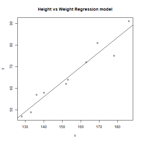
Multiple Regression
Multiple regression is another type of regression analysis technique that is an extension of the linear regression model as it uses more than one predictor variables to create the model. Mathematically,
Implementation in R
Multiple regression in R programming uses the same lm() function to create the model.
Syntax: lm(formula, data)
Parameters:
- formula: represents the formula on which data has to be fitted
- data: represents dataframe on which formula has to be applied
Example: Let us create a multiple regression model of air quality dataset present in R base package and plot the model on the graph.
R
input <- airquality[1:50,
c("Ozone", "Wind", "Temp")]
model <- lm(Ozone~Wind + Temp,
data = input)
cat("Regression model:\n")
print(model)
png(file = "multipleRegGFG.png")
plot(model)
dev.off()
|
Output:
Regression model:
Call:
lm(formula = Ozone ~ Wind + Temp, data = input)

Coefficients:
(Intercept)         Wind         Temp
    -58.239       -0.739        1.329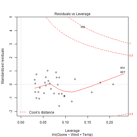
Logistic Regression
Logistic Regression is another widely used regression analysis technique and predicts the value with a range. Moreover, it is used for predicting the values for categorical data. For example, Email is either spam or non-spam, winner or loser, male or female, etc. Mathematically,
where,
- y represents response variable
- z represents equation of independent variables or features
Implementation in R
In R programming, glm() function is used to create a logistic regression model.
Syntax: glm(formula, data, family)
Parameters:
- formula: represents a formula on the basis of which model has to be fitted
- data: represents dataframe on which formula has to be applied
- family: represents the type of function to be used. “binomial” for logistic regression
Example:
R
model <- glm(formula = vs ~ wt,
family = binomial,
data = mtcars)
x <- seq(min(mtcars$wt),
max(mtcars$wt),
0.01)
y <- predict(model, list(wt = x),
type = "response")
print(model)
png(file = "LogRegGFG.png")
plot(mtcars$wt, mtcars$vs, pch = 16,
xlab = "Weight", ylab = "VS")
lines(x, y)
dev.off()
|
Output:
Call:  glm(formula = vs ~ wt, family = binomial, data = mtcars)

Coefficients:
(Intercept)           wt
      5.715       -1.911

Degrees of Freedom: 31 Total (i.e. Null);  30 Residual
Null Deviance:      43.86
Residual Deviance: 31.37        AIC: 35.37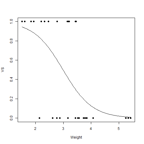
Share your thoughts in the comments
Please Login to comment...