Descriptive Analysis in R Programming

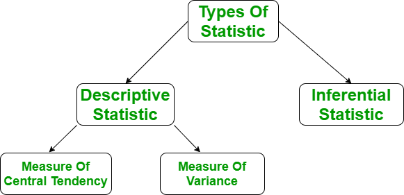
In Descriptive statistics in R Programming Language, we describe our data with the help of various representative methods using charts, graphs, tables, excel files, etc. In the descriptive analysis, we describe our data in some manner and present it in a meaningful way so that it can be easily understood.

Most of the time it is performed on small data sets and this analysis helps us a lot to predict some future trends based on the current findings. Some measures that are used to describe a data set are measures of central tendency and measures of variability or dispersion. 

Process of Descriptive Statistics in R

• The measure of central tendency
• Measure of variability

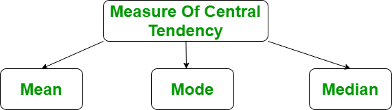
Measure of central tendency

It represents the whole set of data by a single value. It gives us the location of central points. There are three main measures of central tendency: 

• Mean
• Mode
• Median

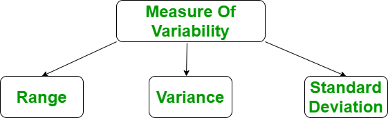
Measure of variability

In Descriptive statistics in R measure of variability is known as the spread of data or how well is our data is distributed. The most common variability measures are: 

• Range
• Variance
• Standard deviation

Need of Descriptive Statistics in R

Descriptive Analysis helps us to understand our data and is a very important part of Machine Learning. This is due to Machine Learning being all about making predictions. On the other hand, statistics is all about drawing conclusions from data, which is a necessary initial step for Machine Learning. Let’s do this descriptive analysis in R.

Descriptive Analysis in R

Descriptive analyses consist of describing simply the data using some summary statistics and graphics. Here, we’ll describe how to compute summary statistics using R software.

Import your data into R:

Before doing any computation, first of all, we need to prepare our data, save our data in external .txt or .csv files and it’s a best practice to save the file in the current directory. After that import, your data into R as follow:

Get the csv file here.

R

# R program to illustrate
# Descriptive Analysis

# Import the data using read.csv()
myData = read.csv("CardioGoodFitness.csv",
                stringsAsFactors = F)
# Print the first 6 rows
print(head(myData))

Output:

   Product Age Gender Education MaritalStatus Usage Fitness Income Miles
1   TM195  18   Male        14        Single     3       4  29562   112
2   TM195  19   Male        15        Single     2       3  31836    75
3   TM195  19 Female        14     Partnered     4       3  30699    66
4   TM195  19   Male        12        Single     3       3  32973    85
5   TM195  20   Male        13     Partnered     4       2  35247    47
6   TM195  20 Female        14     Partnered     3       3  32973    66

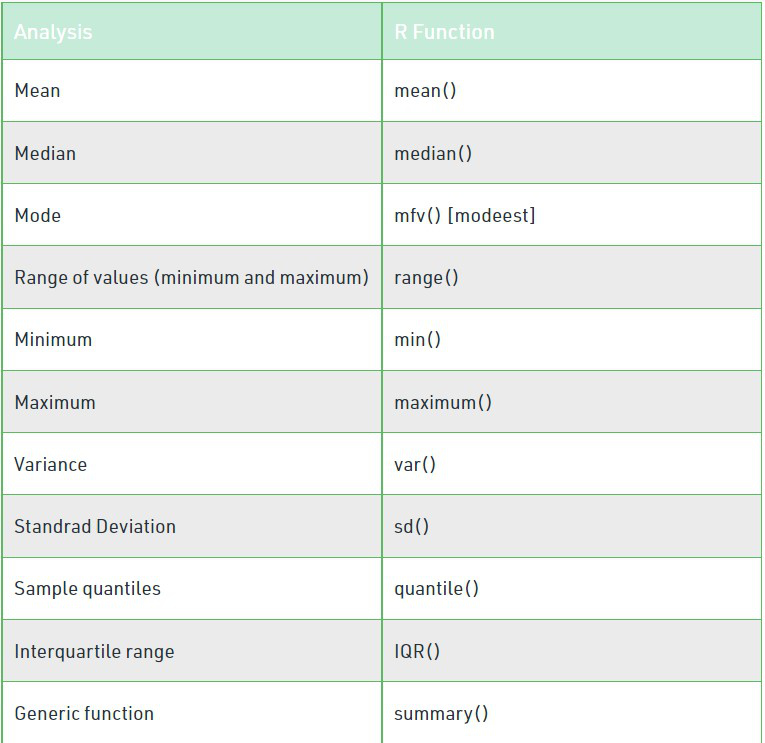
R functions for computing descriptive analysis:

Histogram of Age Distribution

R

library(ggplot2)
ggplot(myData, aes(x = Age)) +
  geom_histogram(binwidth = 2, fill = "blue", color = "red", alpha = 0.8) +
  labs(title = "Age Distribution", x = "Age", y = "Frequency")

Output:

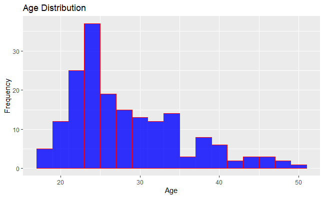
Descriptive Analysis in R Programming

The ggplot2 library to create a histogram of the ‘Age’ variable from the ‘myData’ dataset. The histogram bins have a width of 2, and the bars are filled with a teal color with a light gray border. The resulting visualization shows the distribution of ages in the dataset.

Boxplot of Miles by Gender

R

ggplot(myData, aes(x = Gender, y = Miles, fill = Gender)) +
  geom_boxplot() +
  labs(title = "Miles Distribution by Gender", x = "Gender", y = "Miles") +
  theme_minimal()

Output:

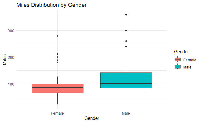
Descriptive Analysis in R Programming

We create a boxplot visualizing the distribution of ‘Miles’ run, segmented by ‘Gender’ from the ‘myData’ dataset. Each boxplot represents the interquartile range (IQR) of Miles for each gender. The plot is titled “Miles Distribution by Gender,” with ‘Gender’ on the x-axis and ‘Miles’ on the y-axis. The plot is styled with a minimal theme.

Bar Chart of Education Levels

R

ggplot(myData, aes(x = factor(Education), fill = factor(Education))) +
  geom_bar() +
  labs(title = "Education Distribution", x = "Education Level", y = "Count") +
  theme_minimal()

Output:

Descriptive Analysis in R Programming

We generate a bar chart illustrating the distribution of ‘Education’ levels from the ‘myData’ dataset. Each bar represents the count of observations for each education level. The chart is titled “Education Distribution,” with ‘Education Level’ on the x-axis and ‘Count’ on the y-axis. The visualization adopts a minimal theme for a clean and simple presentation.

Mean

It is the sum of observations divided by the total number of observations. It is also defined as average which is the sum divided by count.

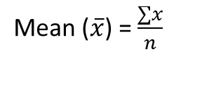
where n = number of terms

R

# R program to illustrate
# Descriptive Analysis

# Import the data using read.csv()
myData = read.csv("CardioGoodFitness.csv",
                stringsAsFactors = F)

# Compute the mean value
mean = mean(myData$Age)
print(mean)

Output:

[1] 28.78889

Median

It is the middle value of the data set. It splits the data into two halves. If the number of elements in the data set is odd then the center element is median and if it is even then the median would be the average of two central elements.

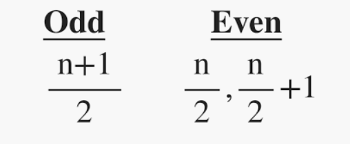
where n = number of terms

R

# R program to illustrate
# Descriptive Analysis

# Import the data using read.csv()
myData = read.csv("CardioGoodFitness.csv",
                stringsAsFactors = F)

# Compute the median value
median = median(myData$Age)
print(median)

Output:

[1] 26

Mode

It is the value that has the highest frequency in the given data set. The data set may have no mode if the frequency of all data points is the same. Also, we can have more than one mode if we encounter two or more data points having the same frequency.

R

# R program to illustrate
# Descriptive Analysis

# Import the library
library(modeest)

# Import the data using read.csv()
myData = read.csv("CardioGoodFitness.csv",
                stringsAsFactors = F)

# Compute the mode value
mode = mfv(myData$Age)
print(mode)

Output:

[1] 25

Range

The range describes the difference between the largest and smallest data point in our data set. The bigger the range, the more is the spread of data and vice versa.

Range = Largest data value – smallest data value 

R

# R program to illustrate
# Descriptive Analysis

# Import the data using read.csv()
myData = read.csv("CardioGoodFitness.csv",
                stringsAsFactors = F)

# Calculate the maximum
max = max(myData$Age)
# Calculate the minimum
min = min(myData$Age)
# Calculate the range
range = max - min

cat("Range is:\n")
print(range)

# Alternate method to get min and max
r = range(myData$Age)
print(r)

Output:

Range is:
[1] 32
[1] 18 50

Variance

It is defined as an average squared deviation from the mean. It is being calculated by finding the difference between every data point and the average which is also known as the mean, squaring them, adding all of them, and then dividing by the number of data points present in our data set.

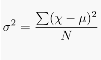
where, 
N = number of terms 
u = Mean

R

# R program to illustrate
# Descriptive Analysis

# Import the data using read.csv()
myData = read.csv("CardioGoodFitness.csv",
                stringsAsFactors = F)

# Calculating variance
variance = var(myData$Age)
print(variance)

Output:

[1] 48.21217

Standard Deviation

It is defined as the square root of the variance. It is being calculated by finding the Mean, then subtract each number from the Mean which is also known as average and square the result. Adding all the values and then divide by the no of terms followed the square root.

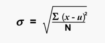
where, 
N = number of terms 
u = Mean

R

# R program to illustrate
# Descriptive Analysis

# Import the data using read.csv()
myData = read.csv("CardioGoodFitness.csv", stringsAsFactors = F)

# Calculating Standard deviation
std = sd(myData$Age)
print(std)

Output:

[1] 6.943498

Some more R function used in Descriptive Statistics in R

Quartiles

A quartile is a type of quantile. The first quartile (Q1), is defined as the middle number between the smallest number and the median of the data set, the second quartile (Q2) – the median of the given data set while the third quartile (Q3), is the middle number between the median and the largest value of the data set.

R

# R program to illustrate
# Descriptive Analysis

# Import the data using read.csv()
myData = read.csv("CardioGoodFitness.csv", stringsAsFactors = F)

# Calculating Quartiles
quartiles = quantile(myData$Age)
print(quartiles)

Output:

0%  25%  50%  75% 100% 
18   24   26   33   50 

Interquartile Range

The interquartile range (IQR), also called as midspread or middle 50%, or technically H-spread is the difference between the third quartile (Q3) and the first quartile (Q1). It covers the center of the distribution and contains 50% of the observations. 

IQR = Q3 – Q1

R

# R program to illustrate
# Descriptive Analysis

# Import the data using read.csv()
myData = read.csv("CardioGoodFitness.csv", stringsAsFactors = F)

# Calculating IQR
IQR = IQR(myData$Age)
print(IQR)

Output:

[1] 9

summary() function in R

The function summary() can be used to display several statistic summaries of either one variable or an entire data frame.

Summary of a single variable:

R

# R program to illustrate
# Descriptive Analysis

# Import the data using read.csv()
myData = read.csv("CardioGoodFitness.csv",
                stringsAsFactors = F)

# Calculating summary
summary = summary(myData$Age)
print(summary)

Output:

 Min. 1st Qu.  Median    Mean 3rd Qu.    Max. 
18.00   24.00   26.00   28.79   33.00   50.00 

Summary of the data frame

R

# R program to illustrate
# Descriptive Analysis

# Import the data using read.csv()
myData = read.csv("CardioGoodFitness.csv",
                stringsAsFactors = F)

# Calculating summary
summary = summary(myData)
print(summary)

Output:

Product               Age           Gender            Education    
 Length:180         Min.   :18.00   Length:180         Min.   :12.00  
 Class :character   1st Qu.:24.00   Class :character   1st Qu.:14.00  
 Mode  :character   Median :26.00   Mode  :character   Median :16.00  
                    Mean   :28.79                      Mean   :15.57  
                    3rd Qu.:33.00                      3rd Qu.:16.00  
                    Max.   :50.00                      Max.   :21.00  
 MaritalStatus          Usage          Fitness          Income           Miles      
 Length:180         Min.   :2.000   Min.   :1.000   Min.   : 29562   Min.   : 21.0  
 Class :character   1st Qu.:3.000   1st Qu.:3.000   1st Qu.: 44059   1st Qu.: 66.0  
 Mode  :character   Median :3.000   Median :3.000   Median : 50597   Median : 94.0  
                    Mean   :3.456   Mean   :3.311   Mean   : 53720   Mean   :103.2  
                    3rd Qu.:4.000   3rd Qu.:4.000   3rd Qu.: 58668   3rd Qu.:114.8  
                    Max.   :7.000   Max.   :5.000   Max.   :104581   Max.   :360.0