Categorical data, representing non-measurable attributes, requires specialized analysis. This article explores descriptive statistics and visualization techniques in R Programming Language for categorical data, focusing on frequencies, proportions, bar charts, pie charts, frequency tables, and contingency tables.
Categorical Data
Categorical data is one of a kind that can be divided into various groups but can not be measured. For example, the income of different persons in a region Rs. 2100, Rs. 1200, etc.- is measurable but the location of those persons Kolkata, Madras, Bangalore, etc.- are categorical data. Categorical data is always discrete.
Descriptive statistics is the idea of quantitatively describing data and one can do that through various means one can do that through visualization techniques like – graphical or tabular representation, etc. If one can deal with categorical datasets, a great way of representing them is by Bar charts, Pie charts, Frequency tables, Contingency tables, etc.
Key Terms for Descriptive Statistics and Visualization in R
- Frequencies: It is nothing but the count of discrete variables that fall into a category.
- For example, we take a categorical data of some customer and there preferences (Y/N) of using black color pen.
- Y stands for ‘Yes’ and N stands for ‘No’.
|
1
|
Y
|
7
|
Y
|
|
2
|
N
|
8
|
N
|
|
3
|
Y
|
9
|
Y
|
|
4
|
Y
|
10
|
N
|
|
5
|
N
|
11
|
N
|
|
6
|
Y
|
12
|
Y
|
Below we simply count the number of customers , fall into one of two category : Y and N
- Frequency Tables: A frequency table gives a view of the number of occurrences of each category of individuals . Example- TABLE-2: categories are Y and N.
- Proportions: A proportion is a way of expressing the fraction of a categorical dataset that has a certain characteristic. It can be written as a ratio, a decimal, or a percentage.
Below, we just take the percentage of each category Y and N, simply by frequency of Y or N divided by Total frequency and multiplied by 100. Here, percentage of Y = (7/12)*100 = 58.33 and, percentage of N = (5/12)*100 = 41.67.
|
Use of Black Pen
|
Percentage
|
|
Y
|
58.33%
|
|
N
|
41.67%
|
- Bar Charts: A bar chart is graphical representation of data that presents a categorical dataset with rectangular bars with heights proportional to the values that they represent. It more use for a categorical data which are ordinal. Types of bar charts- (1) Vertical bar charts: fig1, fig3, fig4, fig5. and (2) Horizontal bar charts: fig2.
- Pie Charts: Pie chart is a representation of percentage distributions in a circular form which divided into parts that are proportional to percentage values. It more use for a categorical data which are nominal.
- Contingency table: It is nothing but a frequency representation of more than one categorical variables. For example we take job interview scenario where some people have a certification on R and work experiences and other have no work experiences or no certification on R or both.
|
1
|
Y
|
N
|
|
2
|
Y
|
Y
|
|
3
|
N
|
Y
|
|
4
|
N
|
N
|
|
5
|
Y
|
N
|
|
6
|
N
|
Y
|
This table shows basically the frequency of (Y,Y), (Y,N), (N,Y) and (N,N). From the above table we can see that the count of (Y,Y) is 1 for person-2 , for person-1 & 5 count of (Y,N) is 2, for person-3 & 6 count of (N,Y) is 2 and for person-4 count of (N,N) is 1. Where Y stands for ‘Yes’ and N stands for ‘No’.
|
Y
|
N
|
|
Y
|
1
|
2
|
3
|
|
N
|
2
|
1
|
3
|
|
Sum/Total
|
3
|
3
|
6
|
In above last row and the last column are basically shows the marginal. Last row represent the work experience wise marginal and last column represent the R certification wise marginal.
- R: Basically, R is programming language which help every statistician to get into their data by some statistical computing and graphical displays.
Prerequisites
Installing Packages and Libraries: To compute these statistical analysis on categorical dataset we need some packages-
- library(ggplot2): Use for generating visualizations
- library(gridExtra): Use for combine multiple plots side by side.
R
install.packages("ggplot2")
install.packages("gridExtra")
library("ggplot2")
library("gridExtra")
library(help=ggplot2)
library(help=gridExtra)
|
Categorical Data Implementation using R
Here we create a most common dataset of smoking status of 380 men and women.
R
set.seed(10)
gender = sample(c('Female', 'Male'), 380, replace = TRUE)
smoking = sample(c('Past smoker', 'Current smoker', 'Non-smoker'), 380, replace = TRUE)
smoker_data = data.frame(gender = as.factor(gender), smoking = as.factor(smoking))
head(smoker_data,10)
|
Output:
   gender        smoking
1  Female    Past smoker
2  Female Current smoker
3    Male    Past smoker
4    Male     Non-smoker
5    Male Current smoker
6  Female Current smoker
7    Male    Past smoker
8    Male     Non-smoker
9  Female Current smoker
10 Female    Past smoker
Calculate count for each combination of categorical variables we can use R’s table() function.
R
table1 = table(smoker_data$gender)
table2 = table(smoker_data$smoking)
print(table1)
print(table2)
|
Output:
Female   Male
   191    189
Current smoker     Non-smoker    Past smoker
           112            128            140
Proportions: To produce the proportions table we simply feed the frequency tables to prop.table() function.
- Proportion table provides a representation of the relative frequencies or proportions of different categories within a dataset.
R
prop.table(table1)
prop.table(table2)
|
Output:
    Female      Male
0.5026316 0.4973684
Current smoker     Non-smoker    Past smoker
     0.2947368      0.3368421      0.3684211
We also create bar plot by using ggplot: Here we try to create first the same bar plot gender wise smoker and smoking status wise and then plot the bar chart by gender wise smoking status which give the clear inside of our created data.
R
gender_data <- as.data.frame(table(smoker_data$gender))
colnames(gender_data) <- c("gender", "count")
smoking_data <- as.data.frame(table(smoker_data$smoking))
colnames(smoking_data) <- c("smoking", "count")
gender_data
smoking_data
|
Output:
    gender count
1 Female   191
2   Male   189

     smoking count
1 Current smoker   112
2     Non-smoker   128
3    Past smoker   140
Visualize the Plots by Gender
R
p1 <- ggplot(gender_data, aes(x = gender, y = count, fill = gender)) +
geom_bar(stat = "identity") +
labs(y = "Number of participants", title = "Distribution by Gender") +
theme_minimal()
print(p1)
|
Output:

Categorical Data Descriptive Statistics in R
Visualize plots Distribution by Smoking Status
R
p2 <- ggplot(smoking_data, aes(x = smoking, y = count, fill = smoking)) +
geom_bar(stat = "identity") +
labs(y = "Number of participants", title = "Distribution by Smoking Status") +
theme_minimal()
p2
|
Output:

Categorical Data Descriptive Statistics in R
Contingency table
To create contingency table we can also use table() function.
R
table(smoker_data$gender,smoker_data$smoking)
|
Output:
         Current smoker Non-smoker Past smoker
  Female             61         61          69
  Male               51         67          71
Marginals
In the context of contingency tables and cross-tabulations, “marginals” refer to the totals found in the margins of the table. Marginals can be classified into two types: row marginals and column marginals.
R
smoking_table <- table(smoker_data$gender, smoker_data$smoking)
marginal_table <- addmargins(smoking_table)
print(marginal_table)
|
Output:
        Current smoker Non-smoker Past smoker Sum
  Female             61         61          69 191
  Male               51         67          71 189
  Sum               112        128         140 380
Now from the above table we can get the row wise and column wise marginal distribution:
R
row_percentages <- prop.table(smoking_table, 1) * 100
col_percentages <- prop.table(smoking_table, 2) * 100
print(row_percentages)
print(col_percentages)
|
Output:
        Current smoker Non-smoker Past smoker
  Female       31.93717   31.93717    36.12565
  Male         26.98413   35.44974    37.56614

         Current smoker Non-smoker Past smoker
  Female       54.46429   47.65625    49.28571
  Male         45.53571   52.34375    50.71429
Pie Charts
Here we first, compute the pie chart by row percentages for each gender and then by column percentages for smoking status for getting more clear understand of the data.
R
library(ggplot2)
library(dplyr)
percentage_data <- smoker_data %>%
group_by(gender, smoking) %>%
summarise(count = n()) %>%
group_by(gender) %>%
mutate(percentage = count / sum(count) * 100)
ggplot(percentage_data, aes(x = "", y = percentage, fill = smoking)) +
geom_bar(width = 1, stat = "identity", position = "fill") +
coord_polar("y") +
geom_text(aes(label = sprintf("%.1f%%", percentage)),
position = position_fill(vjust = 0.5), size = 3) +
labs(title = "Smoking Status Distribution by Gender", fill = "Smoking Status") +
scale_fill_manual(values = c("Past smoker" = "red", "Current smoker" = "pink",
"Non-smoker" = "lightblue")) +
facet_wrap(~ gender) +
theme_void()
|
Output:

Categorical Data Descriptive Statistics in R
In this code, the geom_text layer is used to display the percentages on the pie chart. its also calculated the percentages using the mutate function after the initial summarization.
Here we take a dataset of selling items from kaggle. Here done similar shorts of things.
Here is an example on an External dataset
Dataset Link: Details Dataset
R
df = read.csv("Details.csv")
head(df)
|
Output:
  Order.ID Amount Profit Quantity    Category     Sub.Category PaymentMode
1  B-25681   1096    658        7 Electronics Electronic Games         COD
2  B-26055   5729     64       14   Furniture           Chairs         EMI
3  B-25955   2927    146        8   Furniture        Bookcases         EMI
4  B-26093   2847    712        8 Electronics         Printers Credit Card
5  B-25602   2617   1151        4 Electronics           Phones Credit Card
6  B-25881   2244    247        4    Clothing         Trousers Credit Card
Now here we only operate with categorical columns and draw some perspective from the data by drawing some bar plots using barplot() function , frequency table using table() function and proportion table using prop.table() function:
Frequency tables
R
table1 = table(df$Category)
table2 = table(df$Sub.Category)
table3 = table(df$PaymentMode)
print(table1)
print(table2)
print(table3)
|
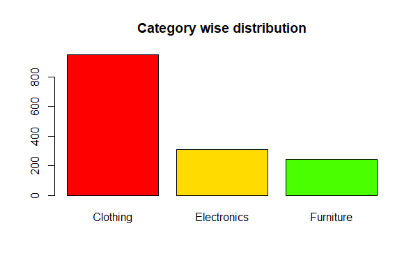
Output:
Clothing Electronics Furniture
949 308 243
Accessories Bookcases Chairs Electronic Games Furnishings
72 79 74 79 73
Hankerchief Kurti Leggings Phones Printers
197 47 53 83 74
Saree Shirt Skirt Stole T-shirt
211 69 64 192 77
Tables Trousers
17 39
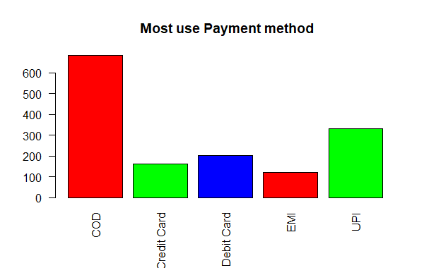
COD Credit Card Debit Card EMI UPI
684 163 202 120 331
Proportion table
R
print(prop.table(table1))
print(prop.table(table2))
print(prop.table(table3))
|
Output:
   Clothing Electronics   Furniture
  0.6326667   0.2053333   0.1620000

     Accessories        Bookcases           Chairs Electronic Games      Furnishings
      0.04800000       0.05266667       0.04933333       0.05266667       0.04866667
     Hankerchief            Kurti         Leggings           Phones         Printers
      0.13133333       0.03133333       0.03533333       0.05533333       0.04933333
           Saree            Shirt            Skirt            Stole          T-shirt
      0.14066667       0.04600000       0.04266667       0.12800000       0.05133333
          Tables         Trousers
      0.01133333       0.02600000

        COD Credit Card  Debit Card         EMI         UPI
  0.4560000   0.1086667   0.1346667   0.0800000   0.2206667
Category wise distribution
R
color <- rainbow(7)
barplot(table(df$Category), main = "Category wise distribution",col = color)
|
Output:
Categorical Data Descriptive Statistics in R
Creating bar plot of category wise sub category
R
table4 <- table(df$Category, df$Sub.Category)
color <- rainbow(nrow(table4))
par(las=2)
bp <- barplot(table4, main = "Category wise distribution", col = color)
legend("topright", legend = rownames(table4),cex = 0.9, fill = color)
axis(1, at=bp, labels=colnames(table4), las=2, cex.axis=1)
|
Output:

Categorical Data Descriptive Statistics in R
R
barplot(table3,main = " Most use Payment method",col= color)
|
Output:
Categorical Data Descriptive Statistics in R
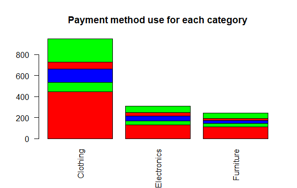
Category wise bar plot stacked by payment method
R
barplot(table(df$PaymentMode, df$Category),
main = "Payment method use for each category", col = color)
legend("topright", unique(df$PaymentMode), cex = 0.7 , fill = color)
|
Output:
Categorical Data Descriptive Statistics in R
Contingency table
R
table4 <- table(df$Category, df$Sub.Category)
print(table4)
|
Output:
              Accessories Bookcases Chairs Electronic Games Furnishings Hankerchief
  Clothing              0         0      0                0           0         197
  Electronics          72         0      0               79           0           0
  Furniture             0        79     74                0          73           0

              Kurti Leggings Phones Printers Saree Shirt Skirt Stole T-shirt Tables
  Clothing       47       53      0        0   211    69    64   192      77      0
  Electronics     0        0     83       74     0     0     0     0       0      0
  Furniture       0        0      0        0     0     0     0     0       0     17

              Trousers
  Clothing          39
  Electronics        0
  Furniture          0
R
table5 <- table(df$PaymentMode,df$Sub.Category,df$Category)
table5
|
Output:
, ,  = Clothing


              Accessories Bookcases Chairs Electronic Games Furnishings Hankerchief
  COD                   0         0      0                0           0          95
  Credit Card           0         0      0                0           0          19
  Debit Card            0         0      0                0           0          28
  EMI                   0         0      0                0           0           7
  UPI                   0         0      0                0           0          48

              Kurti Leggings Phones Printers Saree Shirt Skirt Stole T-shirt Tables
  COD            30       26      0        0    95    31    31    90      33      0
  Credit Card     3        2      0        0    24     6     7    18       5      0
  Debit Card      4       12      0        0    32    11     6    15      12      0
  EMI             2        1      0        0    20     5     2    16       7      0
  UPI             8       12      0        0    40    16    18    53      20      0

              Trousers
  COD               15
  Credit Card        5
  Debit Card         8
  EMI                5
  UPI                6

, ,  = Electronics


              Accessories Bookcases Chairs Electronic Games Furnishings Hankerchief
  COD                  32         0      0               36           0           0
  Credit Card           6         0      0               10           0           0
  Debit Card            7         0      0               12           0           0
  EMI                   8         0      0                8           0           0
  UPI                  19         0      0               13           0           0

              Kurti Leggings Phones Printers Saree Shirt Skirt Stole T-shirt Tables
  COD             0        0     36       24     0     0     0     0       0      0
  Credit Card     0        0     10       15     0     0     0     0       0      0
  Debit Card      0        0     14       14     0     0     0     0       0      0
  EMI             0        0     10        8     0     0     0     0       0      0
  UPI             0        0     13       13     0     0     0     0       0      0

              Trousers
  COD                0
  Credit Card        0
  Debit Card         0
  EMI                0
  UPI                0

, ,  = Furniture


              Accessories Bookcases Chairs Electronic Games Furnishings Hankerchief
  COD                   0        30     37                0          38           0
  Credit Card           0        16     10                0           2           0
  Debit Card            0         6      9                0          11           0
  EMI                   0         9      6                0           3           0
  UPI                   0        18     12                0          19           0

              Kurti Leggings Phones Printers Saree Shirt Skirt Stole T-shirt Tables
  COD             0        0      0        0     0     0     0     0       0      5
  Credit Card     0        0      0        0     0     0     0     0       0      5
  Debit Card      0        0      0        0     0     0     0     0       0      1
  EMI             0        0      0        0     0     0     0     0       0      3
  UPI             0        0      0        0     0     0     0     0       0      3

              Trousers
  COD                0
  Credit Card        0
  Debit Card         0
  EMI                0
  UPI                0
Conclusion
In conclusion, this article demonstrates the power of R in analyzing and visualizing categorical data, providing a comprehensive guide for statisticians. Through practical examples, readers can harness the capabilities of R for descriptive statistics and effective data representation.
Share your thoughts in the comments
Please Login to comment...