DBSCAN Clustering in ML | Density based clustering
Last Updated :
23 May, 2023
Clustering analysis or simply Clustering is basically an Unsupervised learning method that divides the data points into a number of specific batches or groups, such that the data points in the same groups have similar properties and data points in different groups have different properties in some sense. It comprises many different methods based on differential evolution.
E.g. K-Means (distance between points), Affinity propagation (graph distance), Mean-shift (distance between points), DBSCAN (distance between nearest points), Gaussian mixtures (Mahalanobis distance to centers), Spectral clustering (graph distance), etc.
Fundamentally, all clustering methods use the same approach i.e. first we calculate similarities and then we use it to cluster the data points into groups or batches. Here we will focus on the Density-based spatial clustering of applications with noise (DBSCAN) clustering method.
Density-Based Spatial Clustering Of Applications With Noise (DBSCAN)
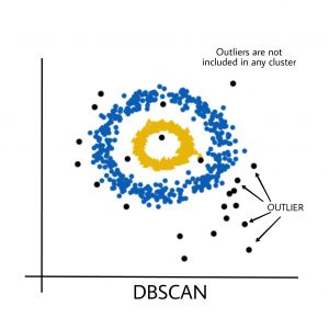
Clusters are dense regions in the data space, separated by regions of the lower density of points. The DBSCAN algorithm is based on this intuitive notion of “clusters” and “noise”. The key idea is that for each point of a cluster, the neighborhood of a given radius has to contain at least a minimum number of points.
Why DBSCAN?
Partitioning methods (K-means, PAM clustering) and hierarchical clustering work for finding spherical-shaped clusters or convex clusters. In other words, they are suitable only for compact and well-separated clusters. Moreover, they are also severely affected by the presence of noise and outliers in the data.
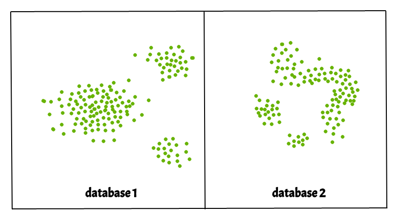
Real-life data may contain irregularities, like:
- Clusters can be of arbitrary shape such as those shown in the figure below.
- Data may contain noise.
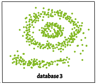
The figure above shows a data set containing non-convex shape clusters and outliers. Given such data, the k-means algorithm has difficulties in identifying these clusters with arbitrary shapes.
Parameters Required For DBSCAN Algorithm
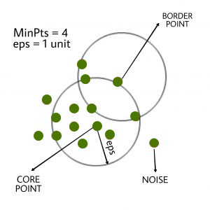
- eps: It defines the neighborhood around a data point i.e. if the distance between two points is lower or equal to ‘eps’ then they are considered neighbors. If the eps value is chosen too small then a large part of the data will be considered as an outlier. If it is chosen very large then the clusters will merge and the majority of the data points will be in the same clusters. One way to find the eps value is based on the k-distance graph.
- MinPts: Minimum number of neighbors (data points) within eps radius. The larger the dataset, the larger value of MinPts must be chosen. As a general rule, the minimum MinPts can be derived from the number of dimensions D in the dataset as, MinPts >= D+1. The minimum value of MinPts must be chosen at least 3.
In this algorithm, we have 3 types of data points.
Core Point: A point is a core point if it has more than MinPts points within eps.
Border Point: A point which has fewer than MinPts within eps but it is in the neighborhood of a core point.
Noise or outlier: A point which is not a core point or border point.
Steps Used In DBSCAN Algorithm
- Find all the neighbor points within eps and identify the core points or visited with more than MinPts neighbors.
- For each core point if it is not already assigned to a cluster, create a new cluster.
- Find recursively all its density-connected points and assign them to the same cluster as the core point.
A point a and b are said to be density connected if there exists a point c which has a sufficient number of points in its neighbors and both points a and b are within the eps distance. This is a chaining process. So, if b is a neighbor of c, c is a neighbor of d, and d is a neighbor of e, which in turn is neighbor of a implying that b is a neighbor of a.
- Iterate through the remaining unvisited points in the dataset. Those points that do not belong to any cluster are noise.
Pseudocode For DBSCAN Clustering Algorithm
DBSCAN(dataset, eps, MinPts){
# cluster index
C = 1
for each unvisited point p in dataset {
         mark p as visited
         # find neighbors
         Neighbors N = find the neighboring points of p

         if |N|>=MinPts:
             N = N U N'
             if p' is not a member of any cluster:
                 add p' to cluster C
}
Implementation Of DBSCAN Algorithm Using Machine Learning In Python
Here, we’ll use the Python library sklearn to compute DBSCAN. We’ll also use the matplotlib.pyplot library for visualizing clusters.
Import Libraries
Python3
import matplotlib.pyplot as plt
import numpy as np
from sklearn.cluster import DBSCAN
from sklearn import metrics
from sklearn.datasets import make_blobs
from sklearn.preprocessing import StandardScaler
from sklearn import datasets
|
Prepare dataset
We will create a dataset using sklearn for modeling. We make_blob for creating the dataset
Python3
X, y_true = make_blobs(n_samples=300, centers=4,
cluster_std=0.50, random_state=0)
|
Modeling The Data Using DBSCAN
Python3
db = DBSCAN(eps=0.3, min_samples=10).fit(X)
core_samples_mask = np.zeros_like(db.labels_, dtype=bool)
core_samples_mask[db.core_sample_indices_] = True
labels = db.labels_
n_clusters_ = len(set(labels)) - (1 if -1 in labels else 0)
unique_labels = set(labels)
colors = ['y', 'b', 'g', 'r']
print(colors)
for k, col in zip(unique_labels, colors):
if k == -1:
col = 'k'
class_member_mask = (labels == k)
xy = X[class_member_mask & core_samples_mask]
plt.plot(xy[:, 0], xy[:, 1], 'o', markerfacecolor=col,
markeredgecolor='k',
markersize=6)
xy = X[class_member_mask & ~core_samples_mask]
plt.plot(xy[:, 0], xy[:, 1], 'o', markerfacecolor=col,
markeredgecolor='k',
markersize=6)
plt.title('number of clusters: %d' % n_clusters_)
plt.show()
|
Output:
.png)
Cluster of dataset
Evaluation Metrics For DBSCAN Algorithm In Machine Learning
We will use the Silhouette score and Adjusted rand score for evaluating clustering algorithms. Silhouette’s score is in the range of -1 to 1. A score near 1 denotes the best meaning that the data point i is very compact within the cluster to which it belongs and far away from the other clusters. The worst value is -1. Values near 0 denote overlapping clusters.
Absolute Rand Score is in the range of 0 to 1. More than 0.9 denotes excellent cluster recovery, and above 0.8 is a good recovery. Less than 0.5 is considered to be poor recovery.
Python3
sc = metrics.silhouette_score(X, labels)
print("Silhouette Coefficient:%0.2f" % sc)
ari = adjusted_rand_score(y_true, labels)
print("Adjusted Rand Index: %0.2f" % ari)
|
Output:
Coefficient:0.13
Adjusted Rand Index: 0.31
Black points represent outliers. By changing the eps and the MinPts, we can change the cluster configuration.
Now the question that should be raised is –
When Should We Use DBSCAN Over K-Means In Clustering Analysis?
DBSCAN(Density-Based Spatial Clustering of Applications with Noise) and K-Means are both clustering algorithms that group together data that have the same characteristic. However, They work on different principles and are suitable for different types of data. We prefer to use DBSCAN when the data is not spherical in shape or the number of classes is not known beforehand.
Difference Between DBSCAN and K-Means.
| DBSCAN |
K-Means |
|
In DBSCAN we need not specify the number
of clusters.
|
K-Means is very sensitive to the number of clusters so it
need to specified
|
| Clusters formed in DBSCAN can be of any arbitrary shape. |
Clusters formed in K-Means are spherical or
convex in shape
|
| DBSCAN can work well with datasets having noise and outliers |
K-Means does not work well with outliers data. Outliers
can skew the clusters in K-Means to a very large extent.
|
| In DBSCAN two parameters are required for training the Model |
In K-Means only one parameter is required is for training
the model
|
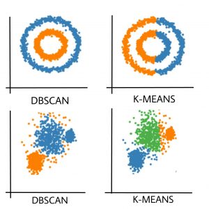
Clusters formed in K-means and DBSCAN
Outlier influence on DBSCAN
More differences between these two algorithms can be found here
Share your thoughts in the comments
Please Login to comment...