Probability Density Estimation & Maximum Likelihood Estimation

Last Updated : 30 May, 2021

Prerequisite: Probability Distribution

Probability Density: Assume a random variable x that has a probability distribution p(x). The relationship between the outcomes of a random variable and its probability is referred to as the probability density.

The problem is that we don’t always know the full probability distribution for a random variable. This is because we only use a small subset of observations to derive the outcome. This problem is referred to as Probability Density Estimation as we use only a random sample of observations to find the general density of the whole sample space.

Probability Density Function (PDF)

A PDF is a function that tells the probability of the random variable from a sub-sample space falling within a particular range of values and not just one value. It tells the likelihood of the range of values in the random variable sub-space being the same as that of the whole sample.

By definition, if X is any continuous random variable, then the function f(x) is called a probability density function if:

$P(a \leq X \leq b) = \int_{a}^{b}f(x)dx$

where,
a -> lower limit
b -> upper limit
X -> continuous random variable
f(x) -> probability density function

Steps Involved:

Step 1 - Create a histogram for the random set of observations to understand the 
         density of the random sample.

Step 2 - Create the probability density function and fit it on the random sample. 
         Observe how it fits the histogram plot.

Step 3 - Now iterate steps 1 and 2 in the following manner:
         3.1 - Calculate the distribution parameters.
          3.2 - Calculate the PDF for the random sample distribution.
         3.3 - Observe the resulting PDF against the data.
         3.4 - Transform the data to until it best fits the distribution.

Most of the histogram of the different random sample after fitting should match the histogram plot of the whole population.

Density Estimation: It is the process of finding out the density of the whole population by examining a random sample of data from that population. One of the best ways to achieve a density estimate is by using a histogram plot.

Parametric Density Estimation

A normal distribution has two given parameters, mean and standard deviation. We calculate the sample mean and standard deviation of the random sample taken from this population to estimate the density of the random sample. The reason it is termed as ‘parametric’ is due to the fact that the relation between the observations and its probability can be different based on the values of the two parameters.

Now, it is important to understand that the mean and standard deviation of this random sample is not going to be the same as that of the whole population due to its small size. A sample plot for parametric density estimation is shown below.

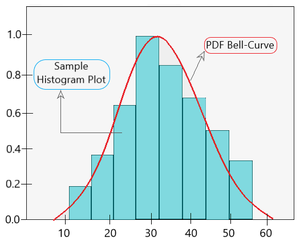
PDF fitted over histogram plot with one peak value

Nonparametric Density Estimation

In some cases, the PDF may not fit the random sample as it doesn’t follow a normal distribution (i.e instead of one peak there are multiple peaks in the graph). Here, instead of using distribution parameters like mean and standard deviation, a particular algorithm is used to estimate the probability distribution. Thus, it is known as a ‘nonparametric density estimation’.

One of the most common nonparametric approach is known as Kernel Density Estimation. In this, the objective is to calculate the unknown density f_h(x) using the equation given below:

$\hat{f}_{h}(x) = \frac{1}{nh} \sum_{i = 1}^{n} K (\frac{x-x_i}{h})$

where,
K -> kernel (non-negative function)
h -> bandwidth (smoothing parameter, h > 0)
K_{h ->} scaled kernel 
f_{h(x) ->} density (to calculate)
n -> no. of samples in random sample.

A sample plot for nonparametric density estimation is given below.

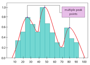
PDF plot over sample histogram plot based on KDE

Problems with Probability Distribution Estimation

Probability Distribution Estimation relies on finding the best PDF and determining its parameters accurately. But the random data sample that we consider, is very small. Hence, it becomes very difficult to determine what parameters and what probability distribution function to use. To tackle this problem, Maximum Likelihood Estimation is used.

Maximum Likelihood Estimation

It is a method of determining the parameters (mean, standard deviation, etc) of normally distributed random sample data or a method of finding the best fitting PDF over the random sample data. This is done by maximizing the likelihood function so that the PDF fitted over the random sample. Another way to look at it is that MLE function gives the mean, the standard deviation of the random sample is most similar to that of the whole sample.

NOTE: MLE assumes that all PDFs are a likely candidate to being the best fitting curve. Hence, it is computationally expensive method.

Intuition:

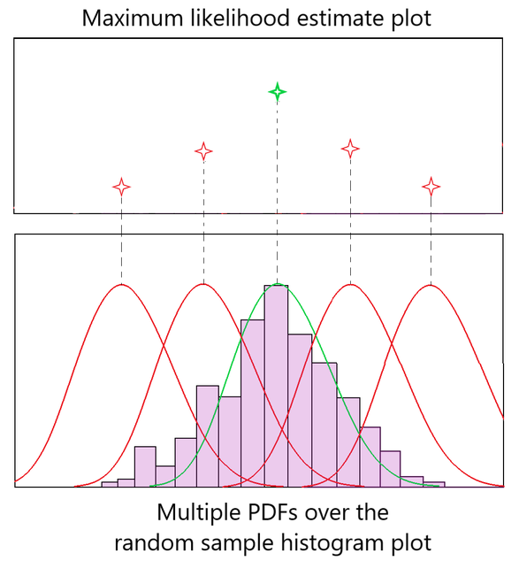
Fig 1 : MLE Intuition

Fig 1 shows multiple attempts at fitting the PDF bell curve over the random sample data. Red bell curves indicate poorly fitted PDF and the green bell curve shows the best fitting PDF over the data. We obtained the optimum bell curve by checking the values in Maximum Likelihood Estimate plot corresponding to each PDF.

As observed in Fig 1, the red plots poorly fit the normal distribution, hence their ‘likelihood estimate’ is also lower. The green PDF curve has the maximum likelihood estimate as it fits the data perfectly. This is how the maximum likelihood estimate method works.

Mathematics Involved

In the intuition, we discussed the role that Likelihood value plays in determining the optimum PDF curve. Let us understand the math involved in MLE method.

We calculate Likelihood based on conditional probabilities. See the equation given below.

$L = F(\ [X_1 = x_1],[X_2 = x_2], ...,[X_n = x_n]\ |\ P) = \Pi_{i = 1}^{n}P^{x_i}(1-P)^{1-x_i}$

where, 
L -> Likelihood value
F -> Probability distribution function
P -> Probability 
X_{1, X2, ... Xn ->} random sample of size n taken from the whole population. 
x_{1, x2, ... xn ->} values that these random sample (Xi) takes when determining the PDF.
Π -> product from 1 to n.

In the above-given equation, we are trying to determine the likelihood value by calculating the joint probability of each X_i taking a specific value x_i involved in a particular PDF. Now, since we are looking for the maximum likelihood value, we differentiate the likelihood function w.r.t P and set it to 0 as given below.

$\frac{\partial L}{\partial P} = 0$

This way, we can obtain the PDF curve that has the maximum likelihood of fit over the random sample data.

But, if you observe carefully, differentiating L w.r.t P is not an easy task as all the probabilities in the likelihood function is a product. Hence, the calculation becomes computationally expensive. To solve this, we take the log of the Likelihood function L.

Log Likelihood

$\log(L) = \log(\Pi_{i = 1}^{n}P^{x_i}(1-P)^{1-x_i})$

Taking the log of likelihood function gives the same result as before due to the increasing nature of Log function. But now, it becomes less computational due to the property of logarithm: $\log{(ab)} = \log{(a)}+\log{(b)}$