Mathematics | Probability Distributions Set 5 (Poisson Distribution)

Last Updated : 09 Mar, 2018

The previous article covered the Binomial Distribution. This article talks about another Discrete Probability Distribution, the Poisson Distribution.

Introduction –

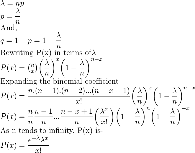
Suppose an event can occur several times within a given unit of time. When the total number of occurrences of the event is unknown, we can think of it as a random variable. This random variable follows the Poisson Distribution. The Poisson distribution is a limiting case of the Binomial distribution when the number of trials becomes very large and the probability of success is small. As we know from the previous article the probability of ‘x’ success in ‘n’ trials in a Binomial Experiment with success probability ‘p’, is- $P(x) = \binom{n}{x} p^x (1-p)^{n-x}$ Let us denote the Expected value of the Random Variable by $\lambda$ .So- $\lambda = np\\ p = \dfrac{\lambda}{n}\\ \text{And, }\\ q = 1-p = 1 - \dfrac{\lambda}{n}\\ \text{Rewriting P(x) in terms of} \lambda\\ P(x) = \binom{n}{x} \bigg(\dfrac{\lambda}{n}\bigg)^x \bigg(1-\dfrac{\lambda}{n}\bigg)^{n-x}\\ \text{Expanding the binomial coefficient}\\ P(x) = \dfrac{n.(n-1).(n-2)...(n-x+1)}{x!} \bigg(\dfrac{\lambda}{n}\bigg)^x \bigg(1-\dfrac{\lambda}{n}\bigg)^{n-x}\\ P(x) = \dfrac{n}{n} \dfrac{n-1}{n}...\dfrac{n-x+1}{n} \bigg(\dfrac{\lambda ^x}{x!}\bigg) \bigg(1-\dfrac{\lambda}{n}\bigg)^{n} \bigg(1-\dfrac{\lambda}{n}\bigg)^{-x}\\ \text{As n tends to infinity, P(x) is-}\\ P(x) = \dfrac{e^{-\lambda} \lambda ^x}{x!}$

Expected Value –

The Expected Value of the Poisson distribution can be found by summing up products of Values with their respective probabilities.

$\begin{flalign*} E[X] &= \sum \limits_{x=0}^{\infty} xp_X(x)\\ &= \sum \limits_{x=0}^{\infty} x\dfrac{e^{-\lambda} \lambda ^x}{x!}\\ &= 0 + \sum \limits_{x=1}^{\infty} x\dfrac{e^{-\lambda} \lambda ^x}{x!} \hspace{3cm}\text{First term is 0 since x=0}\\ &\text{Let x = y + 1}\\ &= \sum \limits_{y=0}^{\infty} (y+1)\dfrac{e^{-\lambda} \lambda ^{y+1}}{(y+1)!}\\ &= \sum \limits_{y=0}^{\infty} (y+1)\dfrac{e^{-\lambda} \lambda ^{y} \lambda}{(y)!(y+1)}\\ &= \lambda \sum \limits_{y=0}^{\infty} \dfrac{e^{-\lambda} \lambda ^{y}}{(y)!}\\ &= \lambda \sum \limits_{y=0}^{\infty} p_Y(y)\\ &= \lambda \end{flalign*}$

Variance and Standard Deviation –

The Variance of the Poisson distribution can be found using the Variance Formula- $Var[X] = E[X^2] - E[X]^2\\$

$\begin{flalign*} E[X^2] &= \sum \limits_{x=0}^{\infty} x^2 p_X(x)\\ &= \sum \limits_{x=0}^{\infty} x^2\dfrac{e^{-\lambda} \lambda ^x}{x!}\\ &= 0 + \sum \limits_{x=1}^{\infty} x^2 \dfrac{e^{-\lambda} \lambda ^x}{x!} \hspace{3cm}\text{First term is 0 since x=0}\\ &\text{Let x = y + 1}\\ &= \sum \limits_{y=0}^{\infty} (y+1)^2\dfrac{e^{-\lambda} \lambda ^{y+1}}{(y+1)!}\\ &= \sum \limits_{y=0}^{\infty} (y+1)^2\dfrac{e^{-\lambda} \lambda ^{y} \lambda}{(y)!(y+1)}\\ &= \lambda \sum \limits_{y=0}^{\infty} (y+1)\dfrac{e^{-\lambda} \lambda ^{y}}{(y)!}\\ &= \lambda \sum \limits_{y=0}^{\infty} (y+1)p_Y(y)\\ &= \lambda \bigg( \sum \limits_{y=0}^{\infty} yp_Y(y) + \sum \limits_{y=0}^{\infty} p_Y(y) \bigg)\\ &= \lambda (\lambda + 1)\\ &= \lambda ^2 + \lambda \end{flalign*}$

Therefore we have Variance as-

$\begin{flalign*} Var[X] &= E[X^2] - E[X]^2\\ &= \lambda^2 + \lambda - \lambda^2\\ &= \lambda \end{flalign*}$

Also the standard Deviation- $\sigma = \sqrt{\lambda}\\$

Relation with Exponential Distribution –

The number of occurrences of an event within a unit of time has a Poisson distribution with parameter $\lambda$ if the time elapsed between two successive occurrences of the event has an exponential distribution with parameter $\lambda$ and it is independent of previous occurrences.

Example- For the case of the thin copper wire, suppose that the number of flaws follows a Poisson distribution with a mean of 2.3 flaws per millimeter. Determine the probability of exactly two flaws in 2 millimeter of wire.
Solution- Let X denote the number of flaws in 1 millimeter of wire. The first step we need to do is to find the parameter $\lambda$ which is nothing but the Expected value of the random variable. In this case we are given the Expected number of flaws in 1 millimeter of wire. We need to find the Expected number of flaws in 2 millimeter of wire. Expected number of flaws in 2 millimeter of wire = 2*np = $2\lambda$ = 2*2.3 = 4.6 Therefore, $P(X=2) = e^{-4.6} \dfrac{(4.6)^2}{2!} = 0.099 \text{ or } 0.1$

GATE CS Corner Questions

Practicing the following questions will help you test your knowledge. All questions have been asked in GATE in previous years or in GATE Mock Tests. It is highly recommended that you practice them. 1. GATE CS 2013, Question 2

References-

Suggest improvement

Mathematics | Probability Distributions Set 4 (Binomial Distribution)

Mathematics | Covariance and Correlation

Share your thoughts in the comments

Matrix and Determinants

Sequence and Series

Calculus

Statistics and Numerical Methods

Probability Distribution

Engineering Math Practice Problems