Mathematics | Probability Distributions Set 2 (Exponential Distribution)

Last Updated : 06 Nov, 2019

The previous article covered the basics of Probability Distributions and talked about the Uniform Probability Distribution. This article covers the Exponential Probability Distribution which is also a Continuous distribution just like Uniform Distribution.

Introduction –

Suppose we are posed with the question- How much time do we need to wait before a given event occurs? The answer to this question can be given in probabilistic terms if we model the given problem using the Exponential Distribution. Since the time we need to wait is unknown, we can think of it as a Random Variable. If the probability of the event happening in a given interval is proportional to the length of the interval, then the Random Variable has an exponential distribution. The support (set of values the Random Variable can take) of an Exponential Random Variable is the set of all positive real numbers. $R_X = [0, \infty)$

Probability Density Function –

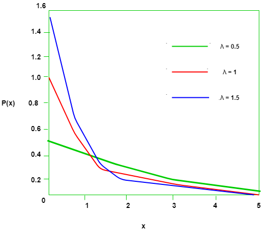
For a positive real number $\lambda$ the probability density function of a Exponentially distributed Random variable is given by-

$f_X(x) = \[ \begin{cases} \lambda e^{-\lambda x} & if x\in R_X 0 \\ 0 & if x \notin R_X \end{cases} \]$

Here $\lambda$ is the rate parameter and its effects on the density function are illustrated below –

To check if the above function is a legitimate probability density function, we need to check if it’s integral over its support is 1.

$\begin{equation*} \begin{split} & = \int\limits_{-\infty}^{\infty} f_X(x) dx \\ & = \int\limits_{0}^{\infty} \lambda e^{-\lambda x} dx \\ & = \frac{\lambda}{-\lambda} \big[ e^{-\lambda x} \big] \limits_{0}^{\infty} \\ & = - \big[ 0 - 1 \big] \\ & = 1 \end{split} \end{equation*}$

Cumulative Density Function –

As we know, the cumulative density function is nothing but the sum of probability of all events upto a certain value of $x = t$ . In the Exponential distribution, the cumulative density function $F(X)$ is given by-

$\begin{equation*} \begin{split} F(X) &= \int\limits_{0}^{t} \lambda e^{-\lambda x} dx \\ &= \big[ \frac{\lambda e^{-\lambda x}}{-\lambda} \big]\limits_{0}^{t} \\ &= \big[ -e^{-\lambda t} + 1 \big]\\ &= 1 -e^{-\lambda t} \end{split} \end{equation*}$

Expected Value –

To find out the expected value, we simply multiply the probability distribution function with x and integrate over all possible values(support).

$\begin{equation*} \begin{split} E[X] & = \int\limits_{-\infty}^{\infty} xf_X(x) dx \\ & = \lambda \int\limits_{0}^{\infty} xe^{-\lambda x} dx \\ & = \lambda \Big\{ \big[ x\int e^{-\lambda x} dx\big]\limits_{0}^{\infty} - \big[ \int \frac{d}{dx} x \big(\int e^{-\lambda x} dx\big)dx \big]\limits_{0}^{\infty} \Big\} \\ & = \lambda \Big\{ \big[ x \frac{e^{-\lambda x}}{-\lambda} \big]\limits_{0}^{\infty} - \big[ \int \frac{e^{-\lambda x}}{-\lambda} dx \big]\limits_{0}^{\infty} \Big\} \\ & = \big[ \frac{-x}{e^{\lambda x}} \big]\limits_{0}^{\infty} + \big[ \int e^{-\lambda x} dx \big]\limits_{0}^{\infty} \\ & = \big[ \frac{-x}{e^{\lambda x}} \big]\limits_{0}^{\infty} + \big[ \frac{e^{-\lambda x}}{-\lambda} \big]\limits_{0}^{\infty} \\ & = \big[ 0-0 \big] - \frac{1}{\lambda} \big[ 0-1 \big] \\ & = \frac{1}{\lambda} \end{split} \end{equation*}$

Variance and Standard deviation –

The variance of the Exponential distribution is given by-

$\begin{equation*} \begin{split} Var[X] &= E[X^2] - E[X]^2\\ & = \int\limits_{-\infty}^{\infty} x^2f_X(x) dx - \frac{1}{\lambda ^2}\\ & = \lambda \int\limits_{0}^{\infty} x^2 e^{-\lambda x} dx - \frac{1}{\lambda ^2}\\ & = \lambda \Big\{ \big[ x^2\int e^{-\lambda x} dx\big]\limits_{0}^{\infty} - \big[ \int \frac{d}{dx} x^2 \big(\int e^{-\lambda x} dx\big)dx \big]\limits_{0}^{\infty} \Big\} - \frac{1}{\lambda ^2}\\ & = \lambda \Big\{ \big[ x^2 \frac{e^{-\lambda x}}{-\lambda} \big]\limits_{0}^{\infty} - \big[ \int 2x\frac{e^{-\lambda x}}{-\lambda} dx \big]\limits_{0}^{\infty} \Big\} - \frac{1}{\lambda ^2}\\ & = \big[ \frac{-x^2}{e^{\lambda x}} \big]\limits_{0}^{\infty} + \frac{2}{\lambda}\big[ \int xe^{-\lambda x} dx \big]\limits_{0}^{\infty} - \frac{1}{\lambda ^2}\\ & = [0-0] + \frac{2}{\lambda} * \frac{1}{\lambda} - \frac{1}{\lambda ^2} \\ & = \frac{2}{\lambda ^2} - \frac{1}{\lambda ^2}\\ & = \frac{1}{\lambda ^2} \end{split} \end{equation*}$

The Standard Deviation of the distribution –

$\begin{equation*} \begin{split} \sigma &= \sqrt{Var[X]}\\ &= \sqrt{\frac{1}{\lambda ^2}}\\ &= \frac{1}{\lambda} \end{split} \end{equation*}$

Example – Let X denote the time between detections of a particle with a Geiger counter and assume that X has an exponential distribution with E(X) = 1.4 minutes. What is the probability that we detect a particle within 30 seconds of starting the counter?
Solution – Since the Random Variable (X) denoting the time between successive detection of particles is exponentially distributed, the Expected Value is given by- $E[X] = \frac{1}{\lambda}$ $\frac{1}{\lambda} = 1.4\\ \lambda = \frac{1}{1.4}$ To find the probability of detecting the particle within 30 seconds of the start of the experiment, we need to use the cumulative density function discussed above. We convert the given 30 seconds in minutes since we have our rate parameter in terms of minutes. $F(0.5) = 1 - e^{\frac{-0.5}{1.4}} \\ F(0.5) = 0.30$

Lack of Memory Property –

Now consider that in the above example, after detecting a particle at the 30 second mark, no particle is detected three minutes since. Because we have been waiting for the past 3 minutes, we feel that a detection is due i.e. the probability of detection of a particle in the next 30 seconds should be higher than 0.3. However. this is not true for the exponential distribution. We can prove so by finding the probability of the above scenario, which can be expressed as a conditional probability- $P(X < 3.5 | X \geq 3) = \frac{P((X < 3.5) \cap (X \geq 3))}{P(X \geq 3)} = \frac{P(3 < X < 3.5)}{P(X \geq 3)}\\\\ P(3 < X < 3.5) = F(3.5) - F(3) = (1 - e^{\frac{-3.5}{1.4}}) - (1 - e^{\frac{-3}{1.4}}) = 0.035 \\\\ P(X \geq 3) = 1 - F(3) = e^{\frac{-3}{1.4}} = 0.117\\\\ P(X < 3.5 | X \geq 3) = \frac{0.035}{0.117} = 0.3$ The fact that we have waited three minutes without a detection does not change the probability of a detection in the next 30 seconds. Therefore, the probability only depends on the length of the interval being considered.

References –

Exponential Distribution Statlect.com

Suggest improvement

Mathematics | Probability Distributions Set 1 (Uniform Distribution)

Mathematics | Probability Distributions Set 3 (Normal Distribution)

Share your thoughts in the comments

Matrix and Determinants

Sequence and Series

Calculus

Statistics and Numerical Methods

Probability Distribution

Engineering Math Practice Problems