Mathematics | Probability Distributions Set 1 (Uniform Distribution)

Prerequisite – Random Variable In probability theory and statistics, a probability distribution is a mathematical function that can be thought of as providing the probabilities of occurrence of different possible outcomes in an experiment. For instance, if the random variable [Tex]X[/Tex] is used to denote the outcome of a coin toss (“the experiment”), then the probability distribution of [Tex]X[/Tex] would take the value 0.5 for [Tex]X[/Tex] = heads, and 0.5 for [Tex]X[/Tex] = tails (assuming the coin is fair). Probability distributions are divided into two classes –

1. Discrete Probability Distribution – If the probabilities are defined on a discrete random variable, one which can only take a discrete set of values, then the distribution is said to be a discrete probability distribution. For example, the event of rolling a die can be represented by a discrete random variable with the probability distribution being such that each event has a probability of [Tex]\:\frac{1}{6}[/Tex].
2. Continuous Probability Distribution – If the probabilities are defined on a continuous random variable, one which can take any value between two numbers, then the distribution is said to be a continuous probability distribution. For example, the temperature throughout a given day can be represented by a continuous random variable and the corresponding probability distribution is said to be continuous.

Cumulative Distribution Function – Similar to the probability density function, the cumulative distribution function [Tex]F(x)[/Tex] of a real-valued random variable X, or just distribution function of [Tex]X[/Tex] evaluated at [Tex]x[/Tex], is the probability that [Tex]X[/Tex] will take a value less than or equal to [Tex]x[/Tex]. For a discrete Random Variable, [Tex] F(x) = P(X\leq x) = \sum \limits_{x_0\leq x} P(x_0) [/Tex] For a continuous Random Variable, [Tex] F(x) = P(X\leq x) = \int \limits_{-\infty}^{x} f(x)dx [/Tex]

Uniform Probability Distribution –

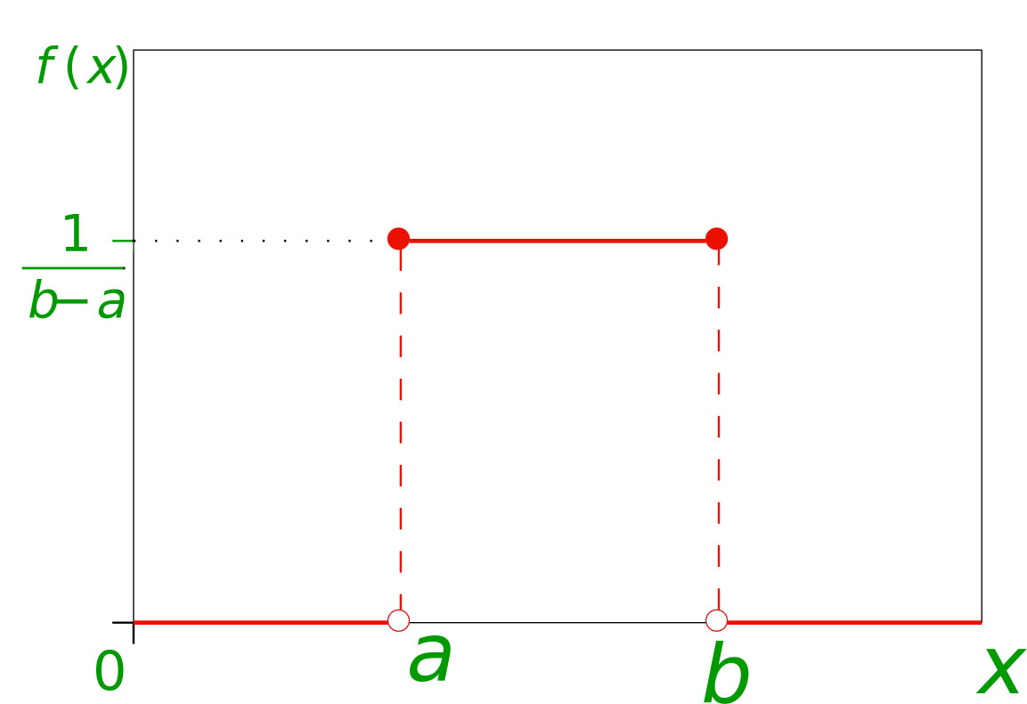
The Uniform Distribution, also known as the Rectangular Distribution, is a type of Continuous Probability Distribution. It has a Continuous Random Variable [Tex]X[/Tex] restricted to a finite interval [Tex][a,b][/Tex] and it’s probability function [Tex]f(x)[/Tex] has a constant density over this interval. The Uniform probability distribution function is defined as- [Tex] f(x) = \begin{cases} \frac{1}{b-a}, & a\leq x \leq b\\ 0, & \text{otherwise}\\ \end{cases} [/Tex] Expected or Mean Value – Using the basic definition of Expectation we get – [Tex] \begin{align*} E(x) &= \int \limits_{-\infty}^{\infty} xf(x) dx&\\ &= \int \limits_{a}^{b} \frac{x}{b-a} dx&\\ &= \frac{1}{b-a} \int \limits_{a}^{b} x dx&\\ &= \frac{1}{b-a} \Big[ \frac{x^2}{2}\Big]_{a}^{b}&\\ &= \frac{b^2 – a^2}{2(b-a)}&\\ &= \frac{b + a}{2}&\\ \end{align*} [/Tex] Variance- Using the formula for variance- [Tex]V(X) = E(X^2) – (E(X))^2[/Tex] [Tex] \begin{align*} E(x^2) &= \int \limits_{-\infty}^{\infty} x^2f(x) dx&\\ &= \int \limits_{a}^{b} \frac{x^2}{b-a} dx&\\ &= \frac{1}{b-a} \int \limits_{a}^{b} x^2 dx&\\ &= \frac{1}{b-a} \Big[ \frac{x^3}{3}\Big]_{a}^{b}&\\ &= \frac{b^3 – a^3}{3(b-a)}&\\ &= \frac{b^2 + a^2 + ab}{3}&\\ \end{align*} [/Tex] Using this result we get – [Tex] \begin{align*} V(x) &= \frac{b^2 + a^2 + ab}{3} – \Big( \frac{b+a}{2}\Big) ^2 &\\ &= \frac{b^2 + a^2 + ab}{3} – \frac{b^2+a^2+2ab}{4} &\\ &= \frac{4b^2 + 4a^2 + 4ab – 3b^2 – 3a^2 – 6ab}{12}&\\ &= \frac{(b-a)^2}{12}&\\ \end{align*} [/Tex] Standard Deviation – By the basic definition of standard deviation, [Tex] \begin{align*} \sigma &= \sqrt{V(x)} \\&= \frac{b-a}{2\sqrt{3}} \end{align*} [/Tex]

• Example 1 – The current (in mA) measured in a piece of copper wire is known to follow a uniform distribution over the interval [0, 25]. Find the formula for the probability density function [Tex]f(x)[/Tex] of the random variable [Tex]X[/Tex] representing the current. Calculate the mean, variance, and standard deviation of the distribution and find the cumulative distribution function [Tex]F(x)[/Tex].
• Solution – The first step is to find the probability density function. For a Uniform distribution, [Tex]f(x) = \frac{1}{b-a}[/Tex], where [Tex]b,\:a[/Tex] are the upper and lower limit respectively. [Tex] \therefore \[ f(x) = \begin{cases} \frac{1}{25-0} = 0.04, & 0\leq x\leq 25 \\ 0, & \text{otherwise} \\ \end{cases} \] [/Tex] The expected value, variance, and standard deviation are- [Tex] E(x) = \frac{b+a}{2} = \frac{25+0}{2} = 12.5 mA\\\\ V(X) = \frac{(b-a)^2}{12} = \frac{(25-0)^2}{12} = 52.08 mA^2\\\\ \text{Standard Deviation} = \sigma = \sqrt{V(x)} = \frac{25}{2\sqrt{3}} = 7.21 mA [/Tex] The cumulative distribution function is given as- [Tex] F(x) = \int \limits_{-\infty}^{x} f(x) dx [/Tex] There are three regions where the CDF can be defined, [Tex]x<0,\: 0\leq x\leq 25,\:25 < x[/Tex] [Tex] \[ F(x) = \begin{cases} 0, &x<0\\ \frac{x}{25}, &0\leq x\leq 25\\ 1, &25<x \end{cases} \] [/Tex]

References –

Probability Distribution – Wikipedia Uniform Probability Distribution – statelect.com