Mathematics | Probability Distributions Set 1 (Uniform Distribution)

Read

Discuss

In probability theory and statistics, a probability distribution is a mathematical function that can be thought of as providing the probabilities of occurrence of different possible outcomes in an experiment. For instance, if the random variable $X$ is used to denote the outcome of a coin toss (“the experiment”), then the probability distribution of $X$ would take the value 0.5 for $X$ = heads, and 0.5 for $X$ = tails (assuming the coin is fair).
Probability distributions are divided into two classes –

Discrete Probability Distribution – If the probabilities are defined on a discrete random variable, one which can only take a discrete set of values, then the distribution is said to be a discrete probability distribution. For example, the event of rolling a die can be represented by a discrete random variable with the probability distribution being such that each event has a probability of $\:\frac{1}{6}$ .
Continuous Probability Distribution – If the probabilities are defined on a continuous random variable, one which can take any value between two numbers, then the distribution is said to be a continuous probability distribution. For example, the temperature throughout a given day can be represented by a continuous random variable and the corresponding probability distribution is said to be continuous.

Cumulative Distribution Function –
Similar to the probability density function, the cumulative distribution function $F(x)$ of a real-valued random variable X, or just distribution function of $X$ evaluated at $x$ , is the probability that $X$ will take a value less than or equal to $x$ .
For a discrete Random Variable,
$F(x) = P(X\leq x) = \sum \limits_{x_0\leq x} P(x_0)$
For a continuous Random Variable,
$F(x) = P(X\leq x) = \int \limits_{-\infty}^{x} f(x)dx$

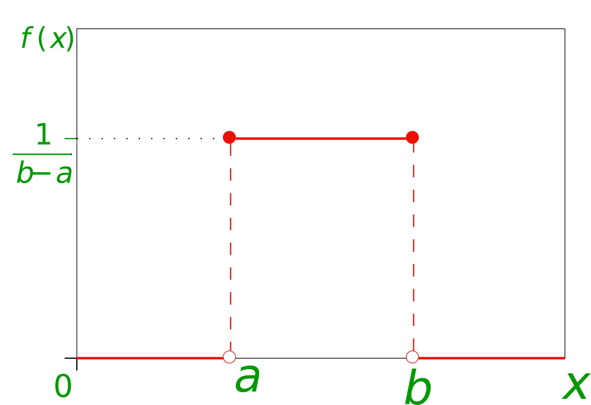
Uniform Probability Distribution –

The Uniform Distribution, also known as the Rectangular Distribution, is a type of Continuous Probability Distribution.
It has a Continuous Random Variable $X$ restricted to a finite interval $[a,b]$ and it’s probability function $f(x)$ has a constant density over this interval.
The Uniform probability distribution function is defined as-

$f(x) = \begin{cases} \frac{1}{b-a}, & a\leq x \leq b\\ 0, & \text{otherwise}\\ \end{cases}$

Uniform Distribution graph

Expected or Mean Value – Using the basic definition of Expectation we get –

$\begin{align*} E(x) &= \int \limits_{-\infty}^{\infty} xf(x) dx&\\ &= \int \limits_{a}^{b} \frac{x}{b-a} dx&\\ &= \frac{1}{b-a} \int \limits_{a}^{b} x dx&\\ &= \frac{1}{b-a} \Big[ \frac{x^2}{2}\Big]_{a}^{b}&\\ &= \frac{b^2 - a^2}{2(b-a)}&\\ &= \frac{b + a}{2}&\\ \end{align*}$

Variance- Using the formula for variance- $V(X) = E(X^2) - (E(X))^2$

$\begin{align*} E(x^2) &= \int \limits_{-\infty}^{\infty} x^2f(x) dx&\\ &= \int \limits_{a}^{b} \frac{x^2}{b-a} dx&\\ &= \frac{1}{b-a} \int \limits_{a}^{b} x^2 dx&\\ &= \frac{1}{b-a} \Big[ \frac{x^3}{3}\Big]_{a}^{b}&\\ &= \frac{b^3 - a^3}{3(b-a)}&\\ &= \frac{b^2 + a^2 + ab}{3}&\\ \end{align*}$

Using this result we get –

$\begin{align*} V(x) &= \frac{b^2 + a^2 + ab}{3} - \Big( \frac{b+a}{2}\Big) ^2 &\\ &= \frac{b^2 + a^2 + ab}{3} - \frac{b^2+a^2+2ab}{4} &\\ &= \frac{4b^2 + 4a^2 + 4ab - 3b^2 - 3a^2 - 6ab}{12}&\\ &= \frac{(b-a)^2}{12}&\\ \end{align*}$

Standard Deviation – By the basic definition of standard deviation,

$\begin{align*} \sigma &= \sqrt{V(x)} \\&= \frac{b-a}{2\sqrt{3}} \end{align*}$

Example 1 – The current (in mA) measured in a piece of copper wire is known to follow a uniform distribution over the interval [0, 25]. Find the formula for the probability density function $f(x)$ of the random variable $X$ representing the current. Calculate the mean, variance, and standard deviation of the distribution and find the cumulative distribution function $F(x)$ .
Solution – The first step is to find the probability density function. For a Uniform distribution, $f(x) = \frac{1}{b-a}$ , where $b,\:a$ are the upper and lower limit respectively.
$\therefore \[ f(x) = \begin{cases} \frac{1}{25-0} = 0.04, & 0\leq x\leq 25 \\ 0, & \text{otherwise} \\ \end{cases} \]$

The expected value, variance, and standard deviation are-
$E(x) = \frac{b+a}{2} = \frac{25+0}{2} = 12.5 mA\\\\ V(X) = \frac{(b-a)^2}{12} = \frac{(25-0)^2}{12} = 52.08 mA^2\\\\ \text{Standard Deviation} = \sigma = \sqrt{V(x)} = \frac{25}{2\sqrt{3}} = 7.21 mA$
The cumulative distribution function is given as-
$F(x) = \int \limits_{-\infty}^{x} f(x) dx$
There are three regions where the CDF can be defined, $x<0,\: 0\leq x\leq 25,\:25 < x$

$F(x) = \begin{cases} 0, &x<0\\ \frac{x}{25}, &0\leq x\leq 25\\ 1, &25<x \end{cases}$

References –

Probability Distribution – Wikipedia
Uniform Probability Distribution – statelect.com

If you like GeeksforGeeks and would like to contribute, you can also write an article using write.geeksforgeeks.org or mail your article to review-team@geeksforgeeks.org. See your article appearing on the GeeksforGeeks main page and help other Geeks.

Please write comments if you find anything incorrect, or you want to share more information about the topic discussed above.

Level Up Your GATE Prep!
Embark on a transformative journey towards GATE success by choosing Data Science & AI as your second paper choice with our specialized course. If you find yourself lost in the vast landscape of the GATE syllabus, our program is the compass you need.

Last Updated : 06 Mar, 2018

Conditional Probability

Mathematics | Probability Distributions Set 2 (Exponential Distribution)

Matrix and Determinants

Sequence and Series

Calculus

Statistics and Numerical Methods

Probability Distribution

Engineering Math Practice Problems