Last Minute Notes – Engineering Mathematics

Last Updated : 28 Oct, 2022

See Last Minute Notes on all subjects here.

Matrices

A matrix represents a collection of numbers arranged in an order of rows and columns. It is necessary to enclose the elements of a matrix in parentheses or brackets.
A matrix with 9 elements is shown below.

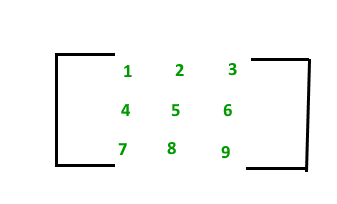
This Matrix [M] has 3 rows and 3 columns. Each element of matrix [M] can be referred to by its row and column number. For example, a₂₃=6

Order of a Matrix :
The order of a matrix is defined in terms of its number of rows and columns.
Order of a matrix = No. of rows ×No. of columns
Therefore Matrix [M] is a matrix of order 3 × 3.

Transpose of a Matrix :
The transpose [M]^T of an m x n matrix [M] is the n x m matrix obtained by interchanging the rows and columns of [M].
if A= [a_ij] mxn , then A^T = [b_ij] nxm where b_ij = a_ji

Properties of transpose of a matrix:

(A^T)^T = A
(A+B)^T = A^T + B^T
(AB)^T = B^TA^T

Singular and Nonsingular Matrix:

Singular Matrix: A square matrix is said to be singular matrix if its determinant is zero i.e. |A|=0
Nonsingular Matrix: A square matrix is said to be non-singular matrix if its determinant is non-zero.

Square Matrix: A square Matrix has as many rows as it has columns. i.e. no of rows = no of columns.
Symmetric matrix: A square matrix is said to be symmetric if the transpose of original matrix is equal to its original matrix. i.e. (A^T) = A.
Skew-symmetric: A skew-symmetric (or antisymmetric or antimetric[1]) matrix is a square matrix whose transpose equals its negative.i.e. (A^T) = -A.
Diagonal Matrix: A diagonal matrix is a matrix in which the entries outside the main diagonal are all zero. The term usually refers to square matrices.
Identity Matrix:A square matrix in which all the elements of the principal diagonal are ones and all other elements are zeros.Identity matrix is denoted as I.
Orthogonal Matrix: A matrix is said to be orthogonal if AA^T = A^TA = I
Idempotent Matrix: A matrix is said to be idempotent if A² = A
Involutory Matrix: A matrix is said to be Involutory if A² = I.

Adjoint of a square matrix:

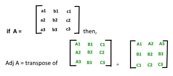
Properties of Adjoint:

A(Adj A) = (Adj A) A = |A| I_n
Adj(AB) = (Adj B).(Adj A)
|Adj A|= |A|^n-1
Adj(kA) = k^n-1 Adj(A)

Inverse of a square matrix:

$A^{-1} = \frac{Adj A}{|A|}$

Here |A| should not be equal to zero, means matrix A should be non-singular.

Properties of inverse:

1. (A^-1)^-1 = A
2. (AB)^-1 = B^-1A^-1
3. Only a non-singular square matrix can have an inverse.

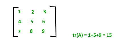
Trace of a matrix :
Let A=[a_ij] _nxn is a square matrix of order n, then the sum of diagonal elements is called the trace of a matrix which is denoted by tr(A). tr(A) = a₁₁ + a₂₂ + a₃₃+ ……….+ a_nn. Remember trace of a matrix is also equal to the sum of eigen value of the matrix. For example:

Properties of trace of matrix:
Let A and B be any two square matrices of order n, then

tr(kA) = k tr(A) where k is a scalar.
tr(A+B) = tr(A)+tr(B)
tr(A-B) = tr(A)-tr(B)
tr(AB) = tr(BA)

Solution of a system of linear equations:
Linear equations can have three kind of possible solutions:

No Solution
Unique Solution
Infinite Solution

Rank of a matrix: Rank of matrix is the number of non-zero rows in the row reduced form or the maximum number of independent rows or the maximum number of independent columns.
Let A be any mxn matrix and it has square sub-matrices of different orders. A matrix is said to be of rank r, if it satisfies the following properties:

It has at least one square sub-matrices of order r who has non-zero determinant.
All the determinants of square sub-matrices of order (r+1) or higher than r are zero.

Rank is denoted as P(A).
if A is a non-singular matrix of order n, then rank of A = n i.e. P(A) = n.

Properties of rank of a matrix:

If A is a null matrix then P(A) = 0 i.e. Rank of null matrix is zero.
If I_n is the nxn unit matrix then P(A) = n.
Rank of a matrix A mxn , P(A) ≤ min(m,n). Thus P(A) ≤m and P(A) ≤ n.
P(A_nxn ) = n if |A| ≠ 0
If P(A) = m and P(B)=n then P(AB) ≤ min(m,n).
If A and B are square matrices of order n then P(AB) ? P(A) + P(B) – n.
If A_m×1 is a non zero column matrix and B_1×n is a non zero row matrix then P(AB) = 1.
The rank of a skew symmetric matrix cannot be equal to one.

System of homogeneous linear equations AX = 0.

X = 0. is always a solution; means all the unknowns has same value as zero. (This is also called trivial solution)
If P(A) = number of unknowns, unique solution.
If P(A) < number of unknowns, infinite number of solutions.

System of non-homogeneous linear equations AX = B.

If P[A:B] ≠P(A), No solution.
If P[A:B] = P(A) = the number of unknown variables, unique solution.
If P[A:B] = P(A) ≠ number of unknown, infinite number of solutions.

Here P[A:B] is rank of gauss elimination representation of AX = B.
There are two states of the Linear equation system:

Consistent State: A System of equations having one or more solutions is called a consistent system of equations.
Inconsistent State: A System of equations having no solutions is called inconsistent system of equations.

Linear dependence and Linear independence of vector:

Linear Dependence: A set of vectors X₁ ,X₂ ….X_r is said to be linearly dependent if there exist r scalars k₁ ,k₂ …..k_r such that: k₁ X₁ + k₂X₂ +……..k_r X_r = 0.

Linear Independence: A set of vectors X₁ ,X₂….X_r is said to be linearly independent if for all r scalars k₁,k₂ …..k_rsuch that k₁X₁+ k₂ X₂+……..k_rX_r = 0, then k₁ = k₂ =……. = k_r = 0.
How to determine linear dependency and independency ?
Let X₁, X₂ ….X_r be the given vectors. Construct a matrix with the given vectors as its rows.

If the rank of the matrix of the given vectors is less than the number of vectors, then the vectors are linearly dependent.
If the rank of the matrix of the given vectors is equal to the number of vectors, then the vectors are linearly independent.

Eigen Value and Eigen Vector

Eigen vector of a matrix A is a vector represented by a matrix X such that when X is multiplied with matrix A, then the direction of the resultant matrix remains the same as vector X.

Mathematically, above statement can be represented as:

AX = λX

where A is any arbitrary matrix, λ are eigen values and X is an eigen vector corresponding to each eigen value.

Here, we can see that AX is parallel to X. So, X is an eigen vector.

Method to find eigen vectors and eigen values of any square matrix A
We know that,

AX = λX

=> AX – λX = 0

=> (A – λI) X = 0 …..(1)

Above condition will be true only if (A – λI) is singular. That means,

|A – λI| = 0 …..(2)

(2) is known as characteristic equation of the matrix.

The roots of the characteristic equation are the eigen values of the matrix A.

Now, to find the eigen vectors, we simply put each eigen value into (1) and solve it by Gaussian elimination, that is, convert the augmented matrix (A – λI) = 0 to row echelon form and solve the linear system of equations thus obtained.

Some important properties of eigen values

Eigen values of real symmetric and hermitian matrices are real
Eigen values of real skew symmetric and skew hermitian matrices are either pure imaginary or zero
Eigen values of unitary and orthogonal matrices are of unit modulus |λ| = 1
If λ_1,=λ₂…….λ_n are the eigen values of A, then kλ₁, kλ₂…….kλ_n are eigen values of kA
If λ_1,λ₂…….λ_n are the eigen values of A, then 1/λ₁, 1/λ₂…….1/λ_n are eigen values of A^-1
If λ_1,λ₂…….λ_n are the eigen values of A, then λ₁^k, λ₂^k…….λ_n^k are eigen values of A^k
Eigen values of A = Eigen Values of A^T(Transpose)
Sum of Eigen Values = Trace of A (Sum of diagonal elements of A)
Product of Eigen Values = |A|
Maximum number of distinct eigen values of A = Size of A
If A and B are two matrices of same order then, Eigen values of AB = Eigen values of BA

Probability

Probability refers to the extent of occurrence of events. When an event occurs like throwing a ball, picking a card from deck, etc ., then the must be some probability associated with that event.

Basic Terminologies:

Random Event :- If the repetition of an experiment occurs several times under similar conditions, if it does not produce the same outcome everytime but the outcome in a trial is one of the several possible outcomes, then such an experiment is called random event or a probabilistic event.
Elementary Event – The elementary event refers to the outcome of each random event performed. Whenever the random event is performed, each associated outcome is known as elementary event.
Sample Space – Sample Space refers to the set of all possible outcomes of a random event.Example, when a coin is tossed, the possible outcomes are head and tail.
Event – An event refers to the subset of the sample space associated with a random event.
Occurrence of an Event – An event associated with a random event is said to occur if any one of the elementary event belonging to it is an outcome.
Sure Event – An event associated with a random event is said to be sure event if it always occurs whenever the random event is performed.
Impossible Event – An event associated with a random event is said to be impossible event if it never occurs whenever the random event is performed.
Compound Event – An event associated with a random event is said to be compound event if it is the disjoint union of two or more elementary events.
Mutually Exclusive Events – Two or more events associated with a random event are said to be mutually exclusive events if any one of the event occurs, it prevents the occurrence of all other events.This means that no two or more events can occur simultaneously at the same time.
Exhaustive Events – Two or more events associated with a random event are said to be exhaustive events if their union is the sample space.

Probability of an Event – If there are total p possible outcomes associated with a random experiment and q of them are favourable outcomes to the event A, then the probability of event A is denoted by P(A) and is given by

 P(A) = q/p

The probability of non occurrence of event A, i.e, P(A’) = 1 – P(A)

Note –

If the value of P(A) = 1, then event A is called sure event .
If the value of P(A) = 0, then event A is called impossible event.
Also, P(A) + P(A’) = 1

Theorems:

General – Let A, B, C are the events associated with a random experiment, then
1. P(A∪B) = P(A) + P(B) – P(A∩B)
2. P(A∪B) = P(A) + P(B) if A and B are mutually exclusive
3. P(A∪B∪C) = P(A) + P(B) + P(C) – P(A∩B) – P(B∩C)- P(C∩A) + P(A∩B∩C)
4. P(A∩B’) = P(A) – P(A∩B)
5. P(A’∩B) = P(B) – P(A∩B)
Extension of Multiplication Theorem – Let A₁, A₂, ….., A_n are n events associated with a random experiment, then P(A₁∩A₂∩A₃ ….. A_n) = P(A₁)P(A₂/A₁)P(A₃/A₂∩A₁) ….. P(A_n/A₁∩A₂∩A₃∩ ….. ∩A_n-1)

Total Law of Probability – Let S be the sample space associated with a random experiment and E₁, E₂, …, E_n be n mutually exclusive and exhaustive events associated with the random experiment . If A is any event which occurs with E₁ or E₂ or … or E_n, then

P(A) = P(E₁)P(A/E₁) + P(E₂)P(A/E₂) + ... +  P(E_n)P(A/E_n)

Conditional Probability

Conditional probability P(A | B) indicates the probability of event ‘A’ happening given that event B happened.

Product Rule:
Derived from above definition of conditional probability by multiplying both sides with P(B)

   P(A ∩ B) = P(B) * P(A|B)

Bayes’s formula
$P(A|B) = \frac{P(B|A)P(A)}{P(B)}$

Random Variables
A random variable is basically a function which maps from the set of sample space to set of real numbers. The purpose is to get an idea about the result of a particular situation where we are given probabilities of different outcomes.

Discrete Probability Distribution – If the probabilities are defined on a discrete random variable, one which can only take a discrete set of values, then the distribution is said to be a discrete probability distribution.

Continuous Probability Distribution – If the probabilities are defined on a continuous random variable, one which can take any value between two numbers, then the distribution is said to be a continuous probability distribution.

Cumulative Distribution Function –
Similar to the probability density function, the cumulative distribution function $F(x)$ of a real-valued random variable X, or just distribution function of $X$ evaluated at $x$ , is the probability that $X$ will take a value less than or equal to $x$ .
For a discrete Random Variable,
$F(x) = P(X\leq x) = \sum \limits_{x_0\leq x} P(x_0)$
For a continuous Random Variable,
$F(x) = P(X\leq x) = \int \limits_{-\infty}^{x} f(x)dx$

Uniform Probability Distribution –

The Uniform Distribution, also known as the Rectangular Distribution, is a type of Continuous Probability Distribution.
It has a Continuous Random Variable $X$ restricted to a finite interval $[a,b]$ and it’s probability function $f(x)$ has a constant density over this interval.
The Uniform probability distribution function is defined as-

$f(x) = \begin{cases} \frac{1}{b-a}, & a\leq x \leq b\\ 0, & \text{otherwise}\\ \end{cases}$

Expectation: The mean of the distribution, represented as E[x].
$E(x) = \int \limits_{-\infty}^{\infty} xf(x) dx\\ or, E[x]=\sum xP(x)$

Variance: $V(X) = E(X^2) - (E(X))^2$ .
For uniform distribution,
$Mean= \frac{b + a}{2}\\$
$Variance= \frac{(b-a)^2}{12}\\$

Exponential Distribution
For a positive real number $\lambda$ the probability density function of a Exponentially distributed Random variable is given by-

$f_X(x) = \[ \begin{cases} \lambda e^{-\lambda x} & if x\in R_X \\ 0 & if x \notin R_X \end{cases} \]$

where R_x is exponential random variables.
$Mean = \frac{1}{\lambda}$
$Variance = \frac{1}{\lambda ^{2}}$

Binomial Distribution:
$P(X=r)=\binom{n}{r}p^{r}(1-p)^{n-r}$
Mean=np, where p is the probability of success
Variance. = np(1-p)

Poisson Distribution:
$P(x) = \dfrac{e^{-\lambda} \lambda ^x}{x!}$
$Mean = \lambda$
$Variance = \lambda$

Calculus:

Limits, Continuity and Differentiability

Existence of Limit – The limit of a function $f(x)$ at $x=a$ exists only when its left hand limit and right hand limit exist and are equal i.e.
$\lim_{x\to a^-}f(x) = \lim_{x\to a^+}f(x)$

Some Common Limits –

$\begin{align*} &\bullet\: \lim_{x\to 0} \frac{\sin x}{x} = 1 \hspace{0.5cm}& &\bullet\: \lim_{x\to 0} \cos x = 1 \hspace{0.5cm}& &\bullet\: \lim_{x\to 0} \frac{\tan x}{x} = 1& \\ &\bullet\: \lim_{x\to 0} \frac{1-\cos x}{x} = 0 \hspace{0.5cm}& &\bullet\: \lim_{x\to 0} \frac{\sin x^\circ}{x} = \frac{\pi}{180} \hspace{0.5cm}& &\bullet\: \lim_{x\to a} \frac{x^n - a^n}{x-a} = na^{n-1}& \\ &\bullet\: \lim_{x\to \infty} (1+\frac{k}{x})^{mx} = e^{mk} \hspace{0.5cm}& &\bullet\: \lim_{x\to 0} (1+x)^\frac{1}{x} = e \hspace{0.5cm}& &\bullet\: \lim_{x\to 0} \frac{(a^x-1)}{x} = \ln {a} \hspace{0.5cm}& \\ &\bullet\: \lim_{x\to 0} \frac{e^x-1}{x} = 1 \hspace{0.5cm}& &\bullet\: \lim_{x\to 0} \frac{\ln {(1+x)}}{x} = 1 \hspace{0.5cm}& &\bullet\: \lim_{x\to \infty} x^\frac{1}{x} = 1 \hspace{0.5cm}& \\ \end{align}$

L’Hospital Rule –
If the given limit $\lim_{x\to a} \frac{f(x)}{g(x)}$ is of the form $\frac{0}{0}$ or $\frac{\infty}{\infty}$ i.e. both $f(x)$ and $g(x)$ are 0 or both $f(x)$ and $g(x)$ are $\infty$ , then the limit can be solved by L’Hospital Rule.
If the limit is of the form described above, then the L’Hospital Rule says that –
$\lim_{x\to a}\frac{f(x)}{g(x)} = \lim_{x\to a}\frac{f^\prime(x)}{g^\prime(x)}$
where $f^\prime(x)$ and $g^\prime(x)$ obtained by differentiating $f(x)$ and $g(x)$ .
If after differentiating, the form still exists, then the rule can be applied continuously until the form is changed.

Continuity
A function is said to be continuous over a range if it’s graph is a single unbroken curve.
Formally,
A real valued function $f(x)$ is said to be continuous at a point $x=x_\circ$ in the domain if –
$\lim_{x\to x_\circ} f(x)$ exists and is equal to $f(x_\circ)$ .
If a function $f(x)$ is continuous at $x=x_\circ$ then-
$\lim_{x\to x_\circ ^+} f(x) = \lim_{x\to x_\circ ^-} f(x) = \lim_{x\to x_\circ} f(x)$
Functions that are not continuous are said to be discontinuous.

Differentiability
The derivative of a real valued function $f(x)$ wrt $x$ is the function $f^\prime(x)$ and is defined as –
$\lim_{h\to 0} \frac{f(x+h)-f(x)}{h}$

A function is said to be differentiable if the derivative of the function exists at all points of its domain. For checking the differentiability of a function at point $x=c$ ,
$\lim_{h\to 0} \frac{f(c+h)-f(c)}{h}$ must exist.

If a function is differentiable at a point, then it is also continuous at that point.
Note – If a function is continuous at a point does not imply that the function is also differentiable at that point. For example, $f(x) = |x|$ is continuous at $x=0$ but it is not differentiable at that point.

Lagrange’s Mean Value Theorem

Suppose $f:[a,b]\rightarrow R$ be a function satisfying three conditions:

1) f(x) is continuous in the closed interval a ≤ x ≤ b

2) f(x) is differentiable in the open interval a < x < b

Then according to Lagrange’s Theorem, there exists at least one point ‘c’ in the open interval (a, b) such that:

$f'(c)=\frac{f(b)-f(a)}{b-a}$

Rolle’s Mean Value Theorem

Suppose f(x) be a function satisfying three conditions:

1) f(x) is continuous in the closed interval a ≤ x ≤ b

2) f(x) is differentiable in the open interval a < x < b

3) f(a) = f(b)

Then according to Rolle’s Theorem, there exists at least one point ‘c’ in the open interval (a, b) such that:

f ‘ (c) = 0

Indefinite Integrals

Definition :Let f(x) be a function. Then the family of all its antiderivatives is called the indefinite integral of a function f(x) and it is denoted by ∫f(x)dx.
The symbol ∫f(x)dx is read as the indefinite integral of f(x) with respect to x.
Thus ∫f(x)dx= ∅(x) + C.
Thus, the process of finding the indefinite integral of a function is called integration of the function.

Fundamental Integration Formulas –

∫xⁿdx = (xⁿ⁺¹/(n+1))+C
∫(1/x)dx = (log_e|x|)+C
∫e^xdx = (e^x)+C
∫a^xdx = ((a^x)/(log_ea))+C
∫sin(x)dx = -cos(x)+C
∫cos(x)dx = sin(x)+C
∫sec²(x)dx = tan(x)+C
∫cosec²(x)dx = -cot(x)+C
∫sec(x)tan(x)dx = sec(x)+C
∫cosec(x)cot(x)dx = -cosec(x)+C
∫cot(x)dx = log|sin(x)|+C
∫tan(x)dx = log|sec(x)|+C
∫sec(x)dx = log|sec(x)+tan(x)|+C
∫cosec(x)dx = log|cosec(x)-cot(x)|+C

Definite Integrals:
Definite integrals are the extension after indefinite integrals, definite integrals have limits [a, b]. It gives the area of a curve bounded between given limits.

$\int_{a}^{b}F(x)dx$ , It denotes the area of curve F(x) bounded between a and b, where a is the lower limit and b is the upper limit.

Note: If f is a continuous function defined on the closed interval [a, b] and F be an anti derivative of f. Then $\int_{a}^{b}f(x)dx= \left [ F(x) \right ]_{a}^{b}\right = F(b)-F(a)$
Here, the function f needs to be well defined and continuous in [a, b].

$\int_{a}^{b}f(x)dx=\int_{a}^{b}f(t)dt$
$\int_{a}^{b}f(x)dx=-\int_{b}^{a}f(x)dx$
$\int_{a}^{b}f(x)dx=\int_{a}^{c}f(x)dx+\int_{c}^{b}f(x)dx$
$\int_{a}^{b}f(x)=\int_{a}^{b}f(a+b-x)dx$
$\int_{0}^{b}f(x)=\int_{0}^{b}f(b-x)dx$
$\int_{0}^{2a}f(x)dx=\int_{0}^{a}f(x)dx+\int_{0}^{a}f(2a-x)dx$
$\int_{-a}^{a}f(x)dx=2\int_{0}^{a}f(x)dx, \textup{if f(x) is even function i.e f(x)=f(-x)}$
$\int_{-a}^{a}f(x)dx=0, \textup{if f(x) is odd function}$