Mathematics | Probability Distributions Set 3 (Normal Distribution)

Last Updated : 31 Oct, 2022

The previous two articles introduced two Continuous Distributions: Uniform and Exponential. This article covers the Normal Probability Distribution, also a Continuous distribution, which is by far the most widely used model for continuous measurement.

Introduction –

Whenever a random experiment is replicated, the Random Variable that equals the average (or total) result over the replicates tends to have a normal distribution as the number of replicates becomes large. It is one of the cornerstones of probability theory and statistics, because of the role it plays in the Central Limit Theorem, and because many real-world phenomena involve random quantities that are approximately normal (e.g., errors in scientific measurement). It is also known by other names such as- Gaussian Distribution, Bell shaped Distribution. 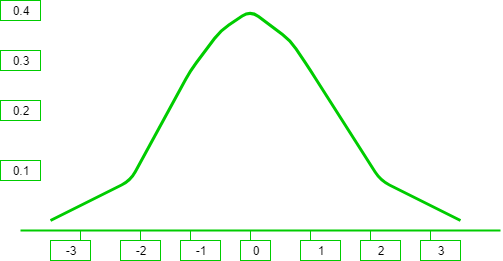It can be observed from the above graph that the distribution is symmetric about its center, which is also the mean (0 in this case). This makes the probability of events at equal deviations from the mean, equally probable. The density is highly centered around the mean, which translates to lower probabilities for values away from the mean.

Probability Density Function –

The probability density function of the general normal distribution is given as- $f_X(x) = \frac{1}{\sigma \sqrt{2\pi}} e^{\frac{-1}{2}\big( \frac{x-\mu}{\sigma} \big)^2}\\$ In the above formula, all the symbols have their usual meanings, $\sigma$ is the Standard Deviation and $\mu$ is the Mean. It is easy to get overwhelmed by the above formula while trying to understand everything in one glance, but we can try to break it down into smaller pieces so as to get an intuition as to what is going on. The z-score is a measure of how many standard deviations away a data point is from the mean. Mathematically, $\text{z-score} = \frac{X-\mu}{\sigma}$ The exponent of $e$ in the above formula is the square of the z-score times $\frac{-1}{2}$ . This is actually in accordance to the observations that we made above. Values away from the mean have a lower probability compared to the values near the mean. Values away from the mean will have a higher z-score and consequently a lower probability since the exponent is negative. The opposite is true for values closer to the mean. This gives way for the 68-95-99.7 rule, which states that the percentage of values that lie within a band around the mean in a normal distribution with a width of two, four and six standard deviations, comprise 68%, 95% and 99.7% of all the values. The figure given below shows this rule- 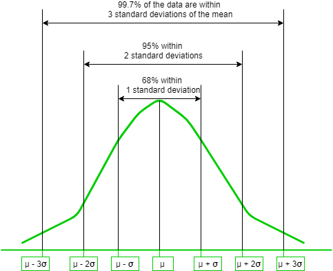The effects of $\mu$ and $\sigma$ on the distribution are shown below. Here $\mu$ is used to reposition the center of the distribution and consequently move the graph left or right, and $\sigma$ is used to flatten or inflate the curve- 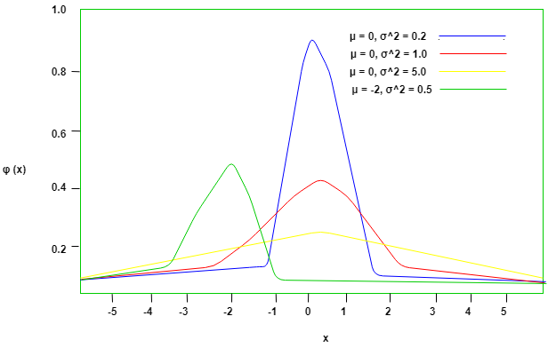Expectation expectation click here or expected value E[x] can be found by simply multiply the probability distribution function with x and integrate over all possible values Let ‘X’ be a normal distributed random variable with parameters $\mu$ ans $\sigma^2$ . we know that area or the region inside normal distribution curve is 1 (because probability is 1) therefore $\int^{+\infty}_{-\infty}f_X(x)\,dx$ = 1 $E[x] = \frac{1}{\sigma \sqrt{2\pi}} $\int^{+\infty}_{-\infty} x*e^{\frac{-1}{2}\big( \frac{x-\mu}{\sigma} \big)^2}\,dx$$ writing x as (x- $\mu$ ) + $\mu$ yields $E[x] = \frac{1}{\sigma \sqrt{2\pi}} $\int^{+\infty}_{-\infty} (x-\mu)*e^{\frac{-1}{2}\big( \frac{x-\mu}{\sigma} \big)^2}\,dx$ + \frac{\mu}{\sigma \sqrt{2\pi}} $\int^{+\infty}_{-\infty} e^{\frac{-1}{2}\big( \frac{x-\mu}{\sigma} \big)^2}\,dx$$ letting y = x- $\mu$ [Tex]E[x] = \frac{1}{\sigma \sqrt{2\pi}} $\int^{+\infty}_{-\infty} y*e^{\frac{-1}{2}\big( \frac{y}{\sigma} \big)^2}\,dx$ + $\mu * \int^{+\infty}_{-\infty}f_X(x)\,dx$ [/Tex]first one is symmetric about y-axis, hence value of that integral is 0. $E[x] = 0 + $\mu * \int^{+\infty}_{-\infty}f_X(x)\,dx$$ [Tex]E[x] = 0 + \mu * 1 [/Tex]therefore , expectation $E[x] = \mu$ variance = $\sigma^2$ standard deviation = $\sqrt{variance} = \sigma$

Standard Normal Distribution –

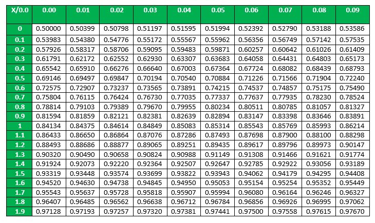
In the General Normal Distribution, if the Mean is set to 0 and the Standard Deviation is set to 1, then the corresponding distribution obtained is called the Standard Normal Distribution. The Probability Density function now becomes- $f_X(x) = \int\limits_{-\infty}^{\infty} \frac{1}{\sigma \sqrt{2\pi}} e^{\frac{-x^2}{2}}$ The cumulative density function of normal distribution does not give a closed formula. Hence precomputed values formulated in tables are used wherever required. But these tables only contain data for the standard distribution. In order to find the cumulative probability for a general normal distribution, it is first standardized and then computed using the value tables. This is beneficial in two ways- 1. First, there needs to be only one table to compute probabilities for all normal distributions. 2. Second, the table size is limited to 40 to 50 rows and 10 columns. This is due 68-95-99.7 rule explained above, which says that values within 3 standard deviations of the mean account for 99.7% probability. So beyond X=3 ( $\mu +3\sigma = 0 + 3*1 = 3$ ) the probabilities are approximately 0.

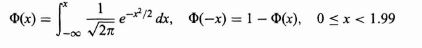
If X is a normal random variable with E(X)= and V(X)=, 
the random variable  is a normal random variable with E(Z)=0 and V(Z)=1. 
That is, Z is a standard normal random variable.

Example – Suppose that the current measurements in a strip of wire are assumed to follow a normal distribution with a mean of 10 milliamperes and a variance of four (milliamperes) $^2$ . What is the probability that a measurement exceeds 13 milliamperes?
Solution – Let X denote the current in milliamperes. The requested probability can be represented as P (X > 13). Let Z = (X ? 10) 2. With the Normal Distribution now standardized, the probability P(X > 13) = P(Z > 1.5) can now be easily computed. Looking at the above table, first we find 1.5 in the X column, and then since there are no more digits of significance we look for 0.00 in the Y column. The corresponding cell gives us the value of $P(Z \leq 1.5) = 0.93319$ So, $P(Z \geq 1.5) = 1 - P(Z \leq 1.5) = 1 - 0.93319 = 0.06681$

Expected value , variance , standard deviation The expected value of a standard normal random variable X is expected value $E[x] = 0$ variance $V[x] = 1$ standard deviation $= 1$

GATE CS Corner Questions

Practicing the following questions will help you test your knowledge. All questions have been asked in GATE in previous years or in GATE Mock Tests. It is highly recommended that you practice them. 1. GATE CS 2008, Question 29

References-

Normal Distribution – Wikipedia 68-95-99.7 Rule

Suggest improvement

Mathematics | Probability Distributions Set 2 (Exponential Distribution)

Mathematics | Probability Distributions Set 4 (Binomial Distribution)

Share your thoughts in the comments

Matrix and Determinants

Sequence and Series

Calculus

Statistics and Numerical Methods

Probability Distribution

Engineering Math Practice Problems