Random Forest Regression in Python

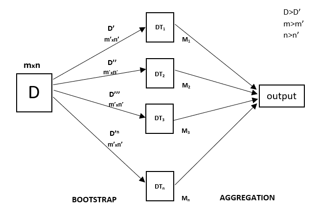
Every decision tree has high variance, but when we combine all of them together in parallel then the resultant variance is low as each decision tree gets perfectly trained on that particular sample data, and hence the output doesn’t depend on one decision tree but on multiple decision trees. In the case of a classification problem, the final output is taken by using the majority voting classifier. In the case of a regression problem, the final output is the mean of all the outputs. This part is called Aggregation. 

Random Forest is an ensemble technique capable of performing both regression and classification tasks with the use of multiple decision trees and a technique called Bootstrap and Aggregation, commonly known as bagging. The basic idea behind this is to combine multiple decision trees in determining the final output rather than relying on individual decision trees. 

Random Forest has multiple decision trees as base learning models. We randomly perform row sampling and feature sampling from the dataset forming sample datasets for every model. This part is called Bootstrap.

We need to approach the Random Forest regression technique like any other machine learning technique 

• Design a specific question or data and get the source to determine the required data.
• Make sure the data is in an accessible format else convert it to the required format.
• Specify all noticeable anomalies and missing data points that may be required to achieve the required data.
• Create a machine-learning model.
• Set the baseline model that you want to achieve
• Train the data machine learning model.
• Provide an insight into the model with test data
• Now compare the performance metrics of both the test data and the predicted data from the model.
• If it doesn’t satisfy your expectations, you can try improving your model accordingly or dating your data, or using another data modeling technique.
• At this stage, you interpret the data you have gained and report accordingly. 

You will be using a similar sample technique in the below example. 

Below is a step-by-step sample implementation of Random Forest Regression, on the dataset that can be downloaded here- https://bit.ly/417n3N5

Implementation:

Step 1: Import the required libraries.

python

# Importing the libraries
import numpy as np
import matplotlib.pyplot as plt
import pandas as pd

Step 2: Import and print the dataset 

python

data = pd.read_csv('Salaries.csv')
print(data)

Output:

Step 3: Select all rows and column 1 from dataset to x and all rows and column 2 as y 

# the coding was not shown which is like that

x= df.iloc [:, : -1] # ” : ” means it will select all rows,    “: -1 ” means that it will ignore last column
y= df.iloc [:, -1 :] # ” : ” means it will select all rows,    “-1 : ” means that it will ignore all columns except the last one

# the “iloc()” function enables us to select a particular cell of the dataset, that is, it helps us select a value that belongs to a particular row or column from a set of values of a data frame or dataset.

Step 4: Fit Random forest regressor to the dataset 

python

# Fitting Random Forest Regression to the dataset
# import the regressor
from sklearn.ensemble import RandomForestRegressor

# create regressor object
regressor = RandomForestRegressor(n_estimators=100, random_state=0)

# fit the regressor with x and y data
regressor.fit(x, y)

Output:

Step 5: Predicting a new result 

python

Y_pred = regressor.predict(np.array([6.5]).reshape(1, 1))  # test the output by changing values

Step 6: Visualising the result

python

# Visualising the Random Forest Regression results

# arrange for creating a range of values
# from min value of x to max
# value of x with a difference of 0.01
# between two consecutive values
X_grid = np.arrange(min(x), max(x), 0.01)

# reshape for reshaping the data into a len(X_grid)*1 array,
# i.e. to make a column out of the X_grid value
X_grid = X_grid.reshape((len(X_grid), 1))

# Scatter plot for original data
plt.scatter(x, y, color = 'blue')

# plot predicted data
plt.plot(X_grid, regressor.predict(X_grid),
         color = 'green')
plt.title('Random Forest Regression')
plt.xlabel('Position level')
plt.ylabel('Salary')
plt.show()

Output:

Out of Bag Score in RandomForest

Bag score or OOB score is the type of validation technique that is mainly used in bagging algorithms to validate the bagging algorithm. Here a small part of the validation data is taken from the mainstream of the data and the predictions on the particular validation data are done and compared with the other results.

The main advantage that the OOB score offers is that here the validation data is not seen by the bagging algorithm and that is why the results on the OOB score are the true results that indicated the actual performance of the bagging algorithm.

To get the OOB score of the particular Random Forest algorithm, one needs to set the value “True” for the OOB_Score parameter in the algorithm. 

Code:

Python3

from sklearn.trees import RandomForestClassifier
RandomeForest = RandomForestClassifier(oob_score=True)
RandomForest.fit(X_train,y_train)
print(RandomForest.oob_score_)

Advantages:

• It is easy to use and less sensitive to the training data compared to the decision tree.
• It is more accurate than the decision tree algorithm.
• It is effective in handling large datasets that have many attributes.
• It can handle missing data, outliers, and noisy features.

Disadvantages:

• The model can also be difficult to interpret.
• This algorithm may require some domain expertise to choose the appropriate parameters like the number of decision trees, the maximum depth of each tree, and the number of features to consider at each split.
• It is computationally expensive, especially for large datasets.
• It may suffer from overfitting if the model is too complex or the number of decision trees is too high.