Isotonic Regression in Scikit Learn

Isotonic regression is a regression technique in which the predictor variable is monotonically related to the target variable. This means that as the value of the predictor variable increases, the value of the target variable either increases or decreases in a consistent, non-oscillating manner.

Mathematically, isotonic regression can be formulated as an optimization problem in which the goal is to find a monotonic function that minimizes the sum of the squared errors between the predicted and observed values of the target variable.

The optimization problem can be written as follows:

minimize  subject to 

where  and  are the predictors and target variables for the  data point, respectively, and f is the monotonic function that is being fit to the data. The constraint ensures that the function is monotonic.

One way to solve this optimization problem is through a dynamic programming approach, which involves iteratively updating the function by adding one predictor-target pair at a time and making sure that the function remains monotonic at each step.

Applications of Isotonic Regression

Isotonic regression has a number of applications, including:

1. Calibration of predicted probabilities: Isotonic regression can be used to adjust the predicted probabilities produced by a classifier so that they are more accurately calibrated to the true probabilities.
2. Ordinal regression: Isotonic regression can be used to model ordinal variables, which are variables that can be ranked in order (e.g., “low,” “medium,” and “high”).
3. Non-parametric regression: Because isotonic regression does not make any assumptions about the functional form of the relationship between the predictor and target variables, it can be used as a non-parametric regression method.
4. Imputing missing values: Isotonic regression can be used to impute missing values in a dataset by predicting the missing values based on the surrounding non-missing values.
5. Outlier detection: Isotonic regression can be used to identify outliers in a dataset by identifying points that are significantly different from the overall trend of the data.

In scikit-learn, isotonic regression can be performed using the ‘IsotonicRegression’ class. This class implements the isotonic regression algorithm, which fits a non-decreasing piecewise-constant function to the data.

Here is an example of how to use the IsotonicRegression class in scikit-learn to perform isotonic regression:

1. Create the sample data with NumPy library

Python3

import numpy as np

# Sample dataset
n=20
x = np.arange(n)
print('Input:\n',x)
y = np.random.randint(0,20,size=n) + 10 * np.log1p(np.arange(n))
print("Target :\n",y)

Outputs :

Input:
 [ 0  1  2  3  4  5  6  7  8  9 10 11 12 13 14 15 16 17 18 19]
Target :
 [ 1.         22.93147181 20.98612289 20.86294361 27.09437912 31.91759469
 38.45910149 23.79441542 22.97224577 35.02585093 32.97895273 40.8490665
 39.64949357 45.3905733  39.08050201 43.72588722 31.33213344 36.90371758
 47.44438979 44.95732274]

2.  Import Isotonic Regression from sklearn.isotonic and predict the Target value

Python3

from sklearn.isotonic import IsotonicRegression
ir = IsotonicRegression() # create an instance of the IsotonicRegression class

# Fit isotonic regression model
y_ir = ir.fit_transform(x, y) # fit the model and transform the data
print('Isotonic Regression Predictions  :\n',y_ir)

Output:

Isotonic Regression Predictions :
 [ 1.         21.59351277 21.59351277 21.59351277 27.09437912 29.28583934
 29.28583934 29.28583934 29.28583934 34.00240183 34.00240183 39.5616248
 39.5616248  39.5616248  39.5616248  39.5616248  39.5616248  39.5616248
 46.20085626 46.20085626]

This code will fit an isotonic regression model to the sample data and make predictions on the same data.  We can observe from the above Target that it is increasing or decreasing along the target value.

3.  Let’s use Linear regression to predict from the same data.

Python3

from sklearn.linear_model import LinearRegression
lr = LinearRegression() # create an instance of the LinearRegression class
# Fit linear regression model
lr.fit(x.reshape(-1, 1), y) # fit the model to the data
y_lr = lr.predict(x.reshape(-1, 1)) # make predictions using the fitted model
print('Linear Regression Prediction :\n', y_lr)

Outputs :

Linear Regression Prediction :
 [17.69949296 19.24352614 20.78755933 22.33159252 23.8756257  25.41965889
 26.96369208 28.50772526 30.05175845 31.59579164 33.13982482 34.68385801
 36.2278912  37.77192438 39.31595757 40.85999076 42.40402394 43.94805713
 45.49209032 47.0361235 ]

4. Let’s compare by plotting both predictions with matplotlib.

Python3

import matplotlib.pyplot as plt
from matplotlib.collections import LineCollection

lines=[[[i,y[i]],[i,y_ir[i]]] for i in range(n)]

# Line to measure the difference between actual and target value
lc=LineCollection(lines)

# plt.figure(figsize=(10,4))
plt.plot(x,y,'.',markersize=10, label='data')
plt.plot(x,y_ir,'-',markersize=10,label='isotonic regression' )
plt.plot(x,y_lr, '-', label='linear regression')

plt.gca().add_collection(lc)
plt.legend() # add a legend

plt.title("Isotonic Regression")
plt.show()

Output: 

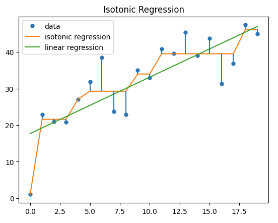
Isotonic Regression

Here, the blue dots represent the original target w.r.t input value. The orange line represents the predicted isotonic regression value. which is varying monotonically along the actual target value. while linear regression is represented by a green line, which is the best linear fit line for input data.

Comparison with different regression algorithms:

Here is a Python code that demonstrates how isotonic regression is different from other regression techniques using a sample dataset:

Python3

from sklearn.preprocessing import PolynomialFeatures
from sklearn.linear_model import LinearRegression
from sklearn.isotonic import IsotonicRegression
import numpy as np
import matplotlib.pyplot as plt

# Sample dataset
n = 20
x = np.arange(n)
print('Input:\n', x)
y = np.random.randint(0, 20, size=n) + 10 * np.log1p(np.arange(n))
print("Target :\n", y)

# Fit isotonic regression model
# create an instance of the IsotonicRegression class
ir = IsotonicRegression()

# fit the model and transform the data
y_ir = ir.fit_transform(x, y)

# Fit linear regression model

# create an instance of the LinearRegression class
lr = LinearRegression()

# fit the model to the data
lr.fit(x.reshape(-1, 1), y)

# make predictions using the fitted model
y_lr = lr.predict(x.reshape(-1, 1))

# Fit polynomial regression model
# create an instance of the PolynomialFeatures
# class with a degree of 2
poly = PolynomialFeatures(degree=2)

# transform the data
x_poly = poly.fit_transform(x.reshape(-1, 1))

# create an instance of the
# LinearRegression class
lr_poly = LinearRegression()

# fit the model to the transformed data
lr_poly.fit(x_poly, y)

# make predictions using the fitted model
y_poly = lr_poly.predict(x_poly)

# Plot the results
plt.plot(x, y, 'o', label='data')  # plot the original data
# plot the fitted isotonic regression model
plt.plot(x, y_ir, label='isotonic regression')
# plot the fitted linear regression model
plt.plot(x, y_lr, label='linear regression')
# plot the fitted polynomial regression model
plt.plot(x, y_poly, label='polynomial regression')
plt.legend()  # add a legend

# Add labels and title
plt.xlabel('X')  # add x-axis label
plt.ylabel('Y')  # add y-axis label
plt.title('Comparison of Regression Techniques')  # add title

plt.show()  # show the plot

Output:

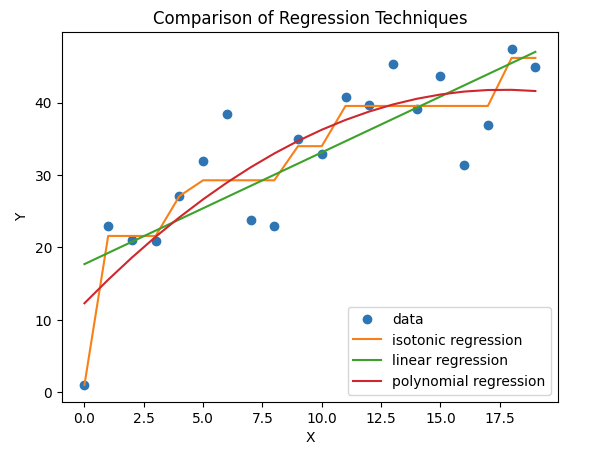
Comparison of different Regression Techniques

The first block imports the necessary libraries and generates a sample dataset with six data points. The second block fits an isotonic regression model to the data using the IsotonicRegression class from the sklearn library. The fit_transform method is used to fit the model and transform the data. The third block fits a linear regression model to the data using the LinearRegression class from the sklearn library. The fourth block fits a polynomial regression model to the data by first transforming the data using the PolynomialFeatures class from the sklearn library, and then fitting a linear regression model to the transformed data. The last block plots the original data, as well as the fitted models, using the matplotlib library.