Ordinary Least Squares and Ridge Regression Variance in Scikit Learn

In statistical modeling, Ordinary Least Squares (OLS) and Ridge Regression are two widely used techniques for linear regression analysis. OLS is a traditional method that finds the line of best fit through the data by minimizing the sum of the squared errors between the predicted and actual values. However, OLS can suffer from high variance and overfitting when the number of predictor variables is large. To address this issue, Ridge Regression introduces a regularization term that shrinks the coefficients toward zero, which can lead to a better model with lower variance.

Concepts related to the topic:

1. Ordinary Least Squares (OLS): ordinary least squares (OLS) is a technique used to calculate the parameters of a linear regression model. The objective is to find the best-fit line that minimizes the sum of squared residuals between the observed data points and the anticipated values from the linear model.
2. Ridge Regression: Ridge Regression is a technique used in linear regression to address the problem of overfitting. It does this by adding a regularization term to the loss function, which shrinks the coefficients toward zero. This reduces the variance of the model and can improve its predictive performance.
3. Regularization: Regularization is a technique used to prevent overfitting in machine learning models. It does this by adding a penalty term to the loss function, which discourages the model from fitting the noise in the data. Regularization can be achieved through methods such as L1 regularization (Lasso), L2 regularization (Ridge), or Elastic Net, depending on the specific problem.
4. Mean Squared Error (MSE): MSE is a metric used to evaluate the performance of regression models. It measures the average of the squared differences between the predicted and actual values. A lower MSE indicates a better fit between the model and the data.
5. R-Squared: R-Squared is a metric used to evaluate the goodness of fit of regression models. It measures the proportion of variance in the dependent variable that is explained by the independent variables. R-Squared ranges from 0 to 1, with higher values indicating a better fit between the model and the data.

Example:

Python3

import numpy as np
import matplotlib.pyplot as plt
from sklearn.preprocessing import PolynomialFeatures
from sklearn.linear_model import LinearRegression, Ridge
from sklearn.metrics import mean_squared_error

# Generate a synthetic dataset with a non-linear relationship
np.random.seed(42)
X = np.linspace(0, 10, 50)
y = np.sin(X) + np.random.normal(0, 0.5, 50)

# Fit OLS and Ridge Regression models with polynomial features
poly = PolynomialFeatures(degree=4)
X_poly = poly.fit_transform(X.reshape(-1, 1))
ols = LinearRegression().fit(X_poly, y)
ridge = Ridge(alpha=1).fit(X_poly, y)

# Predict the output for the test data points
X_test = np.linspace(-2, 12, 100).reshape(-1, 1)
X_test_poly = poly.transform(X_test)
ols_pred = ols.predict(X_test_poly)
ridge_pred = ridge.predict(X_test_poly)

# Compute the mean squared error on the test dataset
ols_mse = mean_squared_error(y_true=y, y_pred=ols.predict(X_poly))
ridge_mse = mean_squared_error(y_true=y, y_pred=ridge.predict(X_poly))

# Plot the data and the regression lines for OLS
plt.scatter(X, y, color='blue', label='Data')
plt.plot(X_test, ols_pred, color='red', label=f'OLS (MSE={ols_mse:.2f})')
plt.legend()
plt.title('Ordinary Least Squares with Polynomial Features')
plt.show()

# Plot the data and the regression lines for Ridge Regression
plt.scatter(X, y, color='blue', label='Data')
plt.plot(X_test, ridge_pred, color='green', label=f'Ridge (MSE={ridge_mse:.2f})')
plt.legend()
plt.title('Ridge Regression with Polynomial Features')
plt.show()

output:

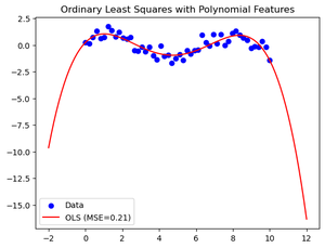
ordinary least square with polynomial feature

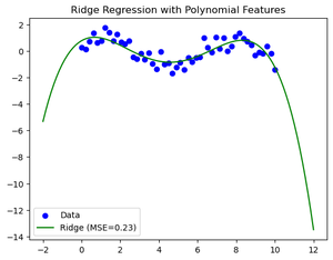
Ridge Regression with Polynomial Features

Ordinary Least Squares and Ridge Regression Variance

Assume we have a dataset containing a response variable, Y, and a predictor variable, X, with n predictors, such as x1, x2, x3,..etc. To predict Y based on predictor X, we want to construct a linear regression model. In this instance, we’ll compare Ridge Regression to the OLS approach.

• Ordinary Least Squares (OLS): OLS aims to minimize the sum of squared residuals and finds the best-fit coefficients for the predictors. The OLS estimator is given by:

• Ridge Regression: Ridge Regression adds a penalty term known as the regularization parameter, to the sum of squared residuals to control the magnitude of the coefficients. The Ridge estimator is given by:

        Here, λ (lambda) is the regularization parameter, and I is the identity matrix

Now, let’s consider the effect of variance in the predictor variables on the coefficients obtained using OLS and Ridge Regression.

Assume that the variance of x1 is significantly larger than the variance of x2. In other words, x1 has a wider range of values compared to x2.

In OLS, the coefficients are estimated using the inverse of (X^T * X), so if one predictor has a larger variance, it will have a greater influence on the estimated coefficients. Consequently, the coefficient for x1 will have a higher variance compared to the coefficient for x2.

In Ridge Regression, the penalty term λ is multiplied by the identity matrix, which helps in shrinking the coefficients towards zero. As a result, Ridge Regression reduces the impact of predictor variables with high variance. Therefore, even if x1 has a higher variance, the Ridge coefficients for x1 and x2 will have a similar variance.

In summary, when there is a difference in variance between predictor variables, OLS tends to give higher variance for coefficients corresponding to predictors with higher variance, while Ridge Regression reduces the variance differences between coefficients by shrinking them towards zero.

Note: The example provided here assumes a simple scenario to demonstrate the variance difference between OLS and Ridge Regression. In practice, the choice between OLS and Ridge Regression depends on various factors, such as the data characteristics, the presence of multicollinearity, and the desired trade-off between bias and variance.

Example:

The code below generates a synthetic dataset with 10 features and 50 samples. We split the data into training and testing sets and fit OLS and Ridge Regression models to the training data. We then compute the mean squared error of the two models on the test dataset and plot the coefficients of the two models to visualize the difference in variance.

Python3

import numpy as np
import matplotlib.pyplot as plt
from sklearn.linear_model import LinearRegression, Ridge
from sklearn.metrics import mean_squared_error

# Generate a synthetic dataset
np.random.seed(23)
X = np.random.normal(size=(50, 10))
y = X.dot(np.random.normal(size=10)) + np.random.random(size=50)

# Split the data into training and testing sets
X_train, X_test, y_train, y_test = X[:40], X[40:], y[:40], y[40:]

# Fit OLS and Ridge Regression models to the training data
ols = LinearRegression().fit(X_train, y_train)
ridge = Ridge(alpha=1.2).fit(X_train, y_train)

# Compute the mean squared error on the test dataset
ols_mse = mean_squared_error(y_true=y_test, y_pred=ols.predict(X_test))
ridge_mse = mean_squared_error(y_true=y_test, y_pred=ridge.predict(X_test))

# Print the mean squared error of the two models
print(f"OLS MSE: {ols_mse:.2f}")
print(f"Ridge MSE: {ridge_mse:.2f}")

# Plot the coefficients of the two models
plt.figure(figsize=(10, 5))
plt.bar(range(X.shape[1]), ols.coef_, color='blue', label='OLS')
plt.bar(range(X.shape[1]), ridge.coef_, color='green', label='Ridge')
plt.xticks(range(X.shape[1]))
plt.legend()
plt.title('Coefficients of OLS and Ridge Regression Models')
plt.show()

Output:

OLS MSE: 0.13 
Ridge MSE: 0.09

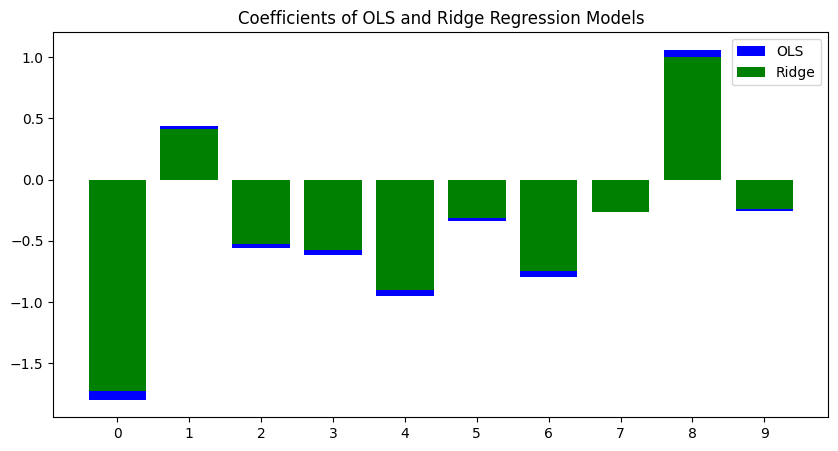
Coefficients of OLS and Ridge Regression Models

The plot shows that compared to the coefficients of the Ridge Regression model, those of the OLS model are bigger in magnitude and have a wider range. As a result, it can be concluded that the OLS model outperforms the Ridge Regression model in terms of variance and sensitivity to data noise.

• OLS Model: The higher MSE of the OLS model (0.13) indicates that it has a relatively higher overall variance compared to the Ridge Regression model.
• Ridge Regression Model: The lower MSE of the Ridge Regression model (0.09) suggests that it has a lower overall variance compared to the OLS model.

The regularisation parameter (lambda) in ridge regression aids in managing the trade-off between minimizing the magnitude of the coefficients and minimising the residual sum of squares. Ridge regression can lessen the variance in the model by adding a penalty term, which lessens overfitting and improves generalisation performance.

As a result, the Ridge Regression model’s lower MSE (0.09) suggests that its variance is lower than that of the OLS model (0.13). This shows that the Ridge Regression model performs better on the dataset in terms of MSE because it is better at eliminating overfitting and capturing the underlying patterns in the data.