Automated Trading using Python
Last Updated :
26 Sep, 2022
Using Python speeds up the trading process, and hence it is also called automated trading/ quantitative trading. The use of Python is credited to its highly functional libraries like TA-Lib, Zipline, Scipy, Pyplot, Matplotlib, NumPy, Pandas etc. Exploring the data at hand is called data analysis. Starting with Python. We will first learn to extract data using the Quandl API.

Using previous data is going to be our key to backtesting strategy. How a strategy works in a given circumstance can only be understood using historical data. We use historical data because in trends in the stock market tend to repeat itself over time.
Setting up work environment
The easiest way to get started is by installing Anaconda. Anaconda is a distribution of Python, and it offers different IDEs like Spyder, Jupyter, __, ___ etc.
Installing Quandl
Quandl will help us in retrieving the historical data of the stock. To install quandl type the below command in the terminal –
pip install quandl
Note: The Quandl Python module is free but you must have a Quandl API key in order to download data. To get your own API key, you will need to create a free Quandl account and set your API key.
Importing packages
Once Quandl is installed, the next step is to import packages. We will be using Pandas rigorously in this tutorial as backtesting requires a lot of data manipulation.
import pandas as pd
import quandl as qd
After the packages have been imported, we will extract data from Quandl, using the API key.
qd.ApiConfig.api_key = "<API key>”
Extracting data using Quandl
Python3
import pandas as pd
import quandl as qd
qd.ApiConfig.api_key = "API KEY"
msft_data = qd.get("EOD/MSFT",
start_date="2010-01-01",
end_date="2020-01-01")
msft_data.head()
|
Output:
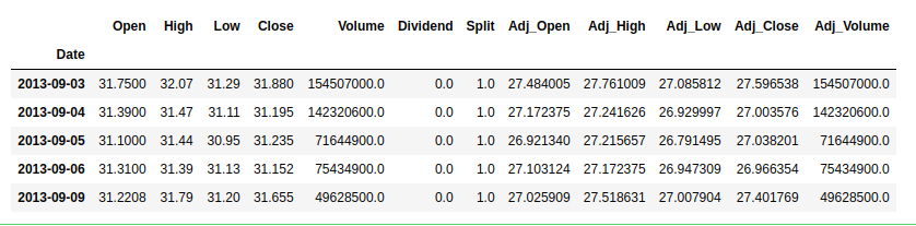
The above code will extract the data of MSFT stocks from 1st Jan 2010 to 1st Jan 2020. data.head() will display first 5 rows of the data.
Important terminology: One should understand what the data represents and depicts.
- Open/ Close – The opening and closing price of the stock.
- High/ Low – The highest and the lowest price the stock has reached during the particular day.
- Adj_High/ Adj_Close – The impact of present dividend distribution, stock splits, or other corporate action on the historical data.
Calculating Returns
Returns is simply the profit gained or losses incurred by the stock after the trader/ investor has used long or short positions. We simply use the function pct_change()
Python3
import numpy as np
close_price = msft_data[['Adj_Close']]
daily_return = close_price.pct_change()
daily_return.fillna(0, inplace=True)
print(daily_return)
|
Output:
            Adj_Close
Date
2013-09-03   0.000000
2013-09-04  -0.021487
2013-09-05   0.001282
2013-09-06  -0.002657
2013-09-09   0.016147
...               ...
2017-12-21  -0.000234
2017-12-22   0.000117
2017-12-26  -0.001286
2017-12-27   0.003630
2017-12-28   0.000117

[1090 rows x 1 columns]
Formula used in daily return = (Price at ‘t’ – Price at 1)/Price at 1 (Price at any given time ‘t’ – opening price)/ opening price
Moving Averages
The concept of moving averages will lay the foundation for our momentum-based trade strategy. For finance, analysts also need to constantly test statistical measures over a sliding time period which is called moving period calculations. Let’s see how the rolling mean can be calculated over a 50-day window, and slide the window by 1 day.
Python3
adj_price = msft_data['Adj_Close']
mav = adj_price.rolling(window=50).mean()
print(mav[-10:])
|
Date
2017-12-14    78.769754
2017-12-15    78.987478
2017-12-18    79.195540
2017-12-19    79.387391
2017-12-20    79.573250
2017-12-21    79.756221
2017-12-22    79.925922
2017-12-26    80.086379
2017-12-27    80.249752
2017-12-28    80.414472
Name: Adj_Close, dtype: float64
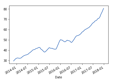
Moving averages help smooth out any data anomalies or spikes, and provide you with a smoother curve for the company’s results.
Plot and see the difference:
Python3
import matplotlib.pyplot as plt
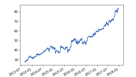
adj_price.plot()
|
Output:
Observe the difference:
Output:
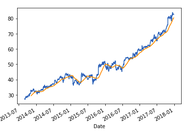
Plotting them together:
Python3
import matplotlib.pyplot as plt
adj_price.plot()
mav.plot()
|
Output:
Share your thoughts in the comments
Please Login to comment...