Python | Decision Tree Regression using sklearn
Last Updated :
11 Jan, 2023
Decision Tree is a decision-making tool that uses a flowchart-like tree structure or is a model of decisions and all of their possible results, including outcomes, input costs, and utility.
Decision-tree algorithm falls under the category of supervised learning algorithms. It works for both continuous as well as categorical output variables.
The branches/edges represent the result of the node and the nodes have either:
- Conditions [Decision Nodes]
- Result [End Nodes]
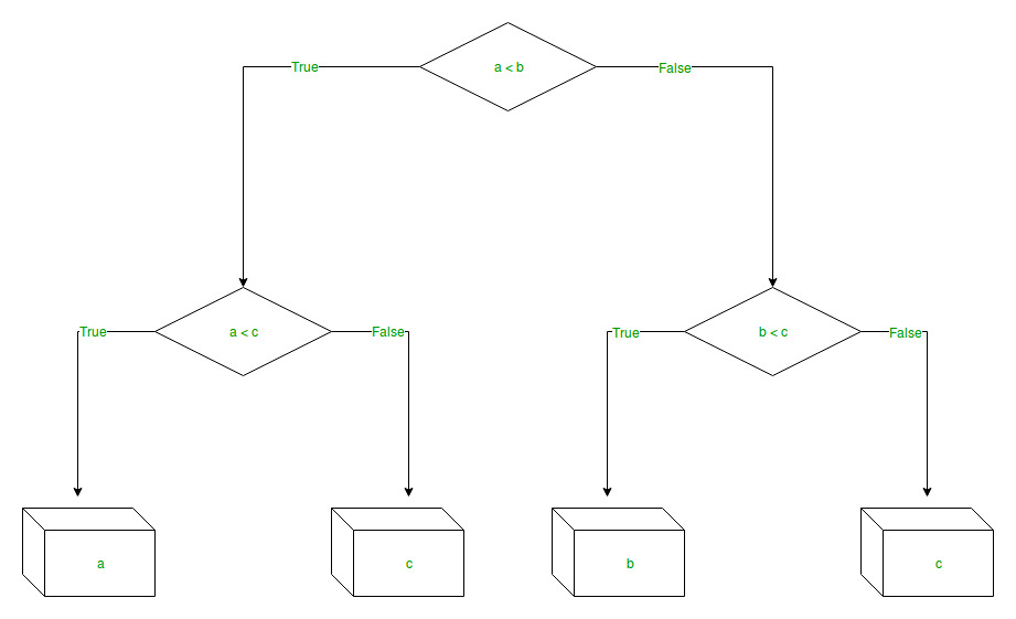
The branches/edges represent the truth/falsity of the statement and take makes a decision based on that in the example below which shows a decision tree that evaluates the smallest of three numbers:
Decision Tree Regression:
Decision tree regression observes features of an object and trains a model in the structure of a tree to predict data in the future to produce meaningful continuous output. Continuous output means that the output/result is not discrete, i.e., it is not represented just by a discrete, known set of numbers or values.
Discrete output example: A weather prediction model that predicts whether or not there’ll be rain on a particular day.
Continuous output example: A profit prediction model that states the probable profit that can be generated from the sale of a product.
Here, continuous values are predicted with the help of a decision tree regression model.
Let’s see the Step-by-Step implementation –
- Step 1: Import the required libraries.
Python3
import numpy as np
import matplotlib.pyplot as plt
import pandas as pd
|
- Step 2: Initialize and print the Dataset.
Python3
dataset = np.array(
[['Asset Flip', 100, 1000],
['Text Based', 500, 3000],
['Visual Novel', 1500, 5000],
['2D Pixel Art', 3500, 8000],
['2D Vector Art', 5000, 6500],
['Strategy', 6000, 7000],
['First Person Shooter', 8000, 15000],
['Simulator', 9500, 20000],
['Racing', 12000, 21000],
['RPG', 14000, 25000],
['Sandbox', 15500, 27000],
['Open-World', 16500, 30000],
['MMOFPS', 25000, 52000],
['MMORPG', 30000, 80000]
])
print(dataset)
|
Output:
[['Asset Flip' '100' '1000']
 ['Text Based' '500' '3000']
 ['Visual Novel' '1500' '5000']
 ['2D Pixel Art' '3500' '8000']
 ['2D Vector Art' '5000' '6500']
 ['Strategy' '6000' '7000']
 ['First Person Shooter' '8000' '15000']
 ['Simulator' '9500' '20000']
 ['Racing' '12000' '21000']
 ['RPG' '14000' '25000']
 ['Sandbox' '15500' '27000']
 ['Open-World' '16500' '30000']
 ['MMOFPS' '25000' '52000']
 ['MMORPG' '30000' '80000']]
- Step 3: Select all the rows and column 1 from the dataset to “X”.
Python3
X = dataset[:, 1:2].astype(int)
print(X)
|
Output:
[[  100]
 [  500]
 [ 1500]
 [ 3500]
 [ 5000]
 [ 6000]
 [ 8000]
 [ 9500]
 [12000]
 [14000]
 [15500]
 [16500]
 [25000]
 [30000]]
- Step 4: Select all of the rows and column 2 from the dataset to “y”.
Python3
y = dataset[:, 2].astype(int)
print(y)
|
Output:
[ 1000 3000 5000 8000 6500 7000 15000 20000 21000 25000 27000 30000 52000 80000]
- Step 5: Fit decision tree regressor to the dataset
Python3
from sklearn.tree import DecisionTreeRegressor
regressor = DecisionTreeRegressor(random_state = 0)
regressor.fit(X, y)
|
Output:
DecisionTreeRegressor(ccp_alpha=0.0, criterion='mse', max_depth=None,
                      max_features=None, max_leaf_nodes=None,
                      min_impurity_decrease=0.0, min_impurity_split=None,
                      min_samples_leaf=1, min_samples_split=2,
                      min_weight_fraction_leaf=0.0, presort='deprecated',
                      random_state=0, splitter='best')
- Step 6: Predicting a new value
Python3
y_pred = regressor.predict([[3750]])
print("Predicted price: % d\n"% y_pred)
|
Output:
Predicted price: 8000
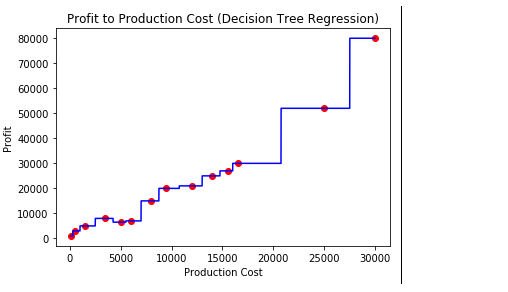
- Step 7: Visualising the result
Python3
X_grid = np.arange(min(X), max(X), 0.01)
X_grid = X_grid.reshape((len(X_grid), 1))
plt.scatter(X, y, color = 'red')
plt.plot(X_grid, regressor.predict(X_grid), color = 'blue')
plt.title('Profit to Production Cost (Decision Tree Regression)')
plt.xlabel('Production Cost')
plt.ylabel('Profit')
plt.show()
|
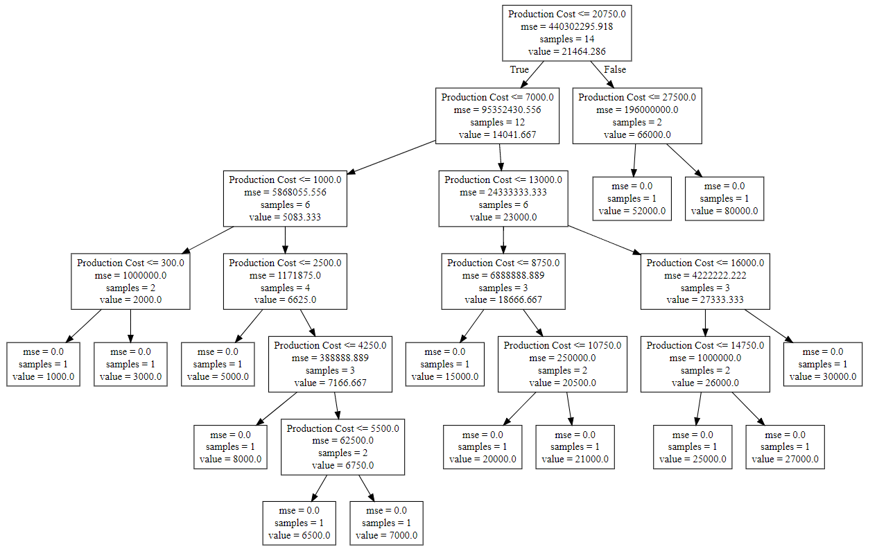
- Step 8: The tree is finally exported and shown in the TREE STRUCTURE below, visualized using http://www.webgraphviz.com/ by copying the data from the ‘tree.dot’ file.
Python3
from sklearn.tree import export_graphviz
export_graphviz(regressor, out_file ='tree.dot',
feature_names =['Production Cost'])
|
Output (Decision Tree):
Share your thoughts in the comments
Please Login to comment...