OpenCV Python Program to analyze an image using Histogram

In this article, image analysis using Matplotlib and OpenCV is discussed. Let’s first understand how to experiment image data with various styles and how to represent with Histogram.
Prerequisites:

• OpenCV
• matplotlib

Importing image data

import matplotlib.pyplot as plt #importing matplotlib

The image should be used in a PNG file as matplotlib supports only PNG images. Here, It’s a 24-bit RGB PNG image (8 bits for each of R, G, B) used in this example. Each inner list represents a pixel. Here, with an RGB image, there are 3 values. For RGB images, matplotlib supports float32 and uint8 data types.

img = plt.imread('flower.png') #reads image data

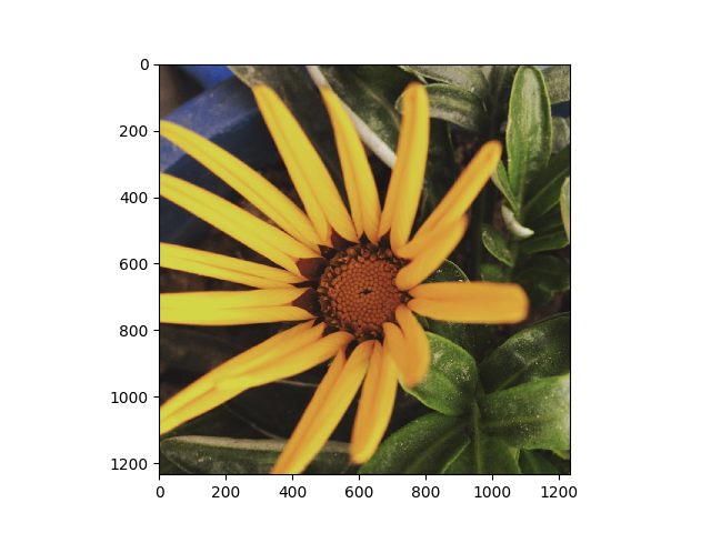
In Matplotlib, this is performed using the imshow() function. Here we have grabbed the plot object.

All about Histogram

Histogram is considered as a graph or plot which is related to frequency of pixels in an Gray Scale Image
with pixel values (ranging from 0 to 255). Grayscale image is an image in which the value of each pixel is a single sample, that is, it carries only intensity information where pixel value varies from 0 to 255. Images of this sort, also known as black-and-white, are composed exclusively of shades of gray, varying from black at the weakest intensity to white at the strongest where Pixel can be considered as a every point in an image.
How GrayScale Image looks like:

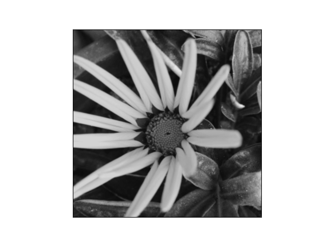
It quantifies the number of pixels for each intensity value considered. Before going through Histogram, lets have a rough idea from this given example.

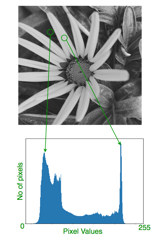
Here, we get intuition about contrast, brightness, intensity distribution etc of that image. As we can see the image and its histogram which is drawn for grayscale image, not color image.
Left region of histogram shows the amount of darker pixels in image and right region shows the amount of brighter pixels.

Histogram creation using numpy array

To create a histogram of our image data, we use the hist() function.

plt.hist(n_img.ravel(), bins=256, range=(0.0, 1.0), fc='k', ec='k') #calculating histogram

In our histogram, it looks like there’s distribution of intensity all over image Black and White pixels as grayscale image.

From the histogram, we can conclude that dark region is more than brighter region.

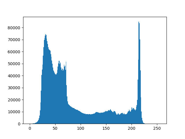
Now, we will deal with an image which  consist of intensity distribution of pixels where pixel value varies. First, we need to calculate histogram using OpenCV in-built function.

Histogram Calculation

Here, we use cv2.calcHist()(in-built function in OpenCV) to find the histogram.

cv2.calcHist(images, channels, mask, histSize, ranges[, hist[, accumulate]])

images : it is the source image of type uint8 or float32 represented as “[img]”.
channels : it is the index of channel for which we calculate histogram. For grayscale image, its value is [0] and
color image, you can pass [0], [1] or [2] to calculate histogram of blue, green or red channel respectively.
mask : mask image. To find histogram of full image, it is given as “None”.
histSize : this represents our BIN count. For full scale, we pass [256].
ranges : this is our RANGE. Normally, it is [0,256].

For example:

# load an image in grayscale mode
img = cv2.imread('ex.jpg',0)

# calculate frequency of pixels in range 0-255
histg = cv2.calcHist([img],[0],None,[256],[0,256])

Then, we need to plot histogram to show the characteristics of an image.

Plotting Histograms

Analysis using Matplotlib:

# importing required libraries of opencv
import cv2

# importing library for plotting
from matplotlib import pyplot as plt

# reads an input image
img = cv2.imread('ex.jpg',0)

# find frequency of pixels in range 0-255
histr = cv2.calcHist([img],[0],None,[256],[0,256])

# show the plotting graph of an image
plt.plot(histr)
plt.show()

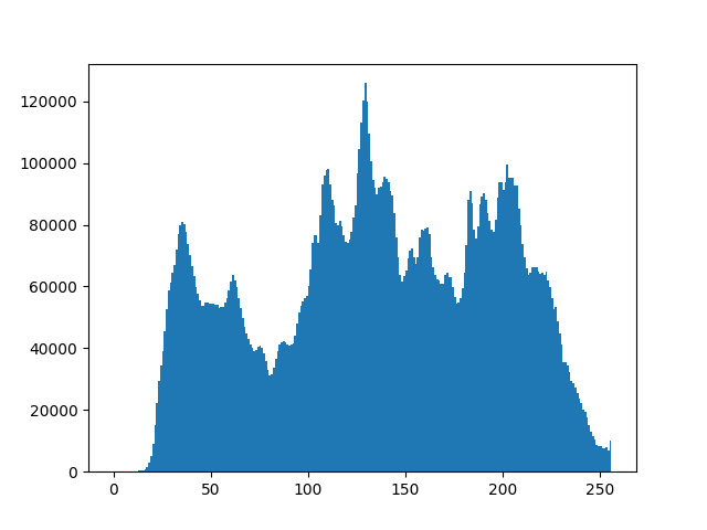
Input:



Output:



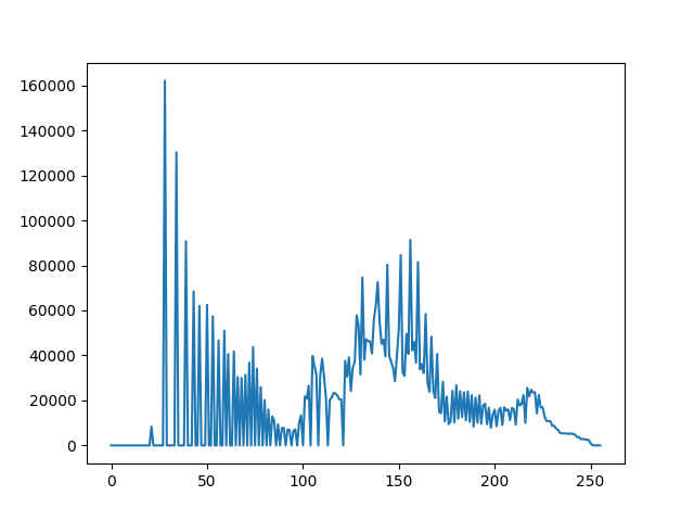
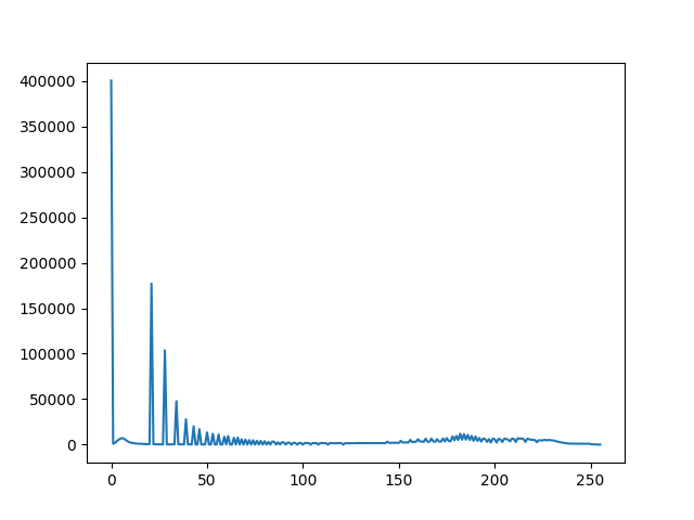
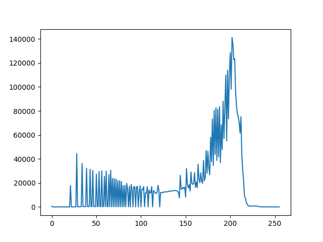
Illustration shows that each number of pixels of an image lie upon range of 0 to 255. In the second example, it directly finds the histogram and plot it. We need not use calcHist(). See the code below:

import cv2
from matplotlib import pyplot as plt
img = cv2.imread('ex.jpg',0)

# alternative way to find histogram of an image
plt.hist(img.ravel(),256,[0,256])
plt.show()

Output:

Thus, we conclude that image can be represented as a Histogram to conceive the idea of intensity distribution over an image and further its tranquility.

References:

• http://docs.opencv.org/2.4/doc/tutorials/imgproc/table_of_content_imgproc/table_of_content_imgproc.html#table-of-content-imgproc
• http://www.cambridgeincolour.com/tutorials/histograms1.htm

If you like GeeksforGeeks and would like to contribute, you can also write an article using write.geeksforgeeks.org or mail your article to review-team@geeksforgeeks.org. See your article appearing on the GeeksforGeeks main page and help other Geeks.

Please write comments if you find anything incorrect, or you want to share more information about the topic discussed above.