GrowNet: Gradient Boosting Neural Networks

Last Updated : 05 Dec, 2022

GrowNet was proposed in 2020 by students from Purdue, UCLA, and Virginia Tech in collaboration with engineers from Amazon and LinkedIn California. They proposed a new gradient boosting algorithm where they used a shallow neural network as the weak learners, a general loss function for training the gradient boosting models under classification, regression, and learning to rank, and a fully corrective step to deal with pitfalls of gradient training and provide stability to it.

Before going on to the architectural details of the GrowNet, it is a prerequisite to have a quick revision at the Gradient Boosting.

Gradient Boosting

Gradient Boosting is a popular boosting algorithm. In gradient boosting, each predictor corrects its predecessor’s error. In contrast to Adaboost, the weights of the training instances are not tweaked, instead, each predictor is trained using the residual errors of predecessor as labels.

There is a technique called the Gradient Boosted

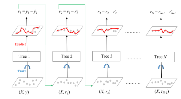
Trees whose base learner is CART (Classification and Regression Trees). The diagram explains how gradient boosted trees are trained for regression problems.

The ensemble consists of N trees. Tree1 is trained using the feature matrix X and the labels y. The predictions labelled $\hat{y}$ are used to determine the training set residual errors $r_2$ . Tree2 is then trained using the feature matrix X and the residual errors $r_1$ of Tree1 as labels. The predicted results $\hat{r_1}$ are then used to determine the residual $r_2$ . The process is repeated until all the N trees forming the ensemble are trained.

Architecture

As we learned above that the key idea behind the Gradient Boosting algorithm is to take the simple, lower-order model as a kind of building block to build a more powerful, higher-order model by sequential boosting using first or second-order gradient statistics. In the Grownet, we use shallow neural networks (e.g., with one or two hidden layers) as weak learners.

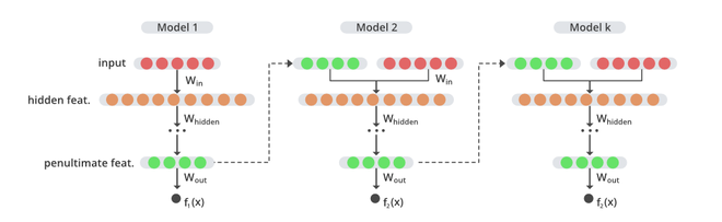
GrowNet architecture

In every boosting step, we combine the vectors of the original input features with output from the last layer of the current iteration. This new feature-set is then passed as input to train the next weak learner via boosting algorithm using current residuals. The final output of the model is a weighted combination of scores from all these sequentially trained weak learner models.

Let’s assume a dataset with n samples and d dimensional feature space D ={(x_i, y_i)_{i=1}^{n} | x_i \epsilon R^{d}, y_i \epsilon R}. Grownet uses K additive functions to predict the output:

$\hat{y_i} = \varepsilon(x_i) = \sum_{k=0}^{K} a_k f_k (x_i), f_k \epsilon F$

where, f_k represents an independent, shallow weak learner with linear layer as output layer, a_k is the step size (boost rate).

Here, our objective function that the shallow learner need to minimize is following:

$L(\varepsilon) = \sum_{i=0}^{n} l(y_i, \hat{y_i})$

However, this objective function will not be enough because as similar to Gradient Boosting Decision Trees, the model is trained on an additive manner. Therefore, we need to add the output of the previous stage for sample $x_i$ . Now, the output of the previous stage is:

$\hat{y_i}^{(t-1)} = \sum_{k = 0}^{t-1} a_k f_k (x_i)$

Therefore our objective function for stage t becomes:

$L^{(t)} = \sum_{i=0}^{n} l(y_i, \hat{y}_i^{(t-1)} + \alpha_t f_t(x_i))$

The above objective function can be simplified as:

$L^{(t)} = \sum_{i=0}^{n} h(\widetilde{y_i} - \alpha_t f_t(x_i))^{2}$

where, \widetilde{y_i} = -\frac{g_i}{h_i}, and g_i and h_i are first order gradient of objective function l at x_iwrt \hat{y}_i^{t-1}. In the next step, we will be calculating the value of g and h for regression, classification and rank learning:

Regression

For regression, Let’s consider we apply the mse loss function and take l to represent it, then the formula for calculating different variables at stage t are:

$g_i = 2(\hat{y_i}^{(t-1)} - y_i ) \\ \\ \\ h_i =2 ; \widetilde{y_i} = y_i - y_i^{(t-1)}$

Now, for the next weak learner f_t by least square regression on \left \{ x_i, \widetilde{y_i} \right \} for i =1, 2, 3, …. n. In the corrective step, all model parameters are back-propagated using MSE loss.

Classification

Let’s consider binary cross entropy loss as our loss function for the classification and labels such as y_i \epsilon {\left \{-1,1 \right \}} .This is because y_i^2 = 1 which can be used in our derivation. then the formula for calculating different variables at stage t are as follows:

$g_i = \frac{-2 y_i}{(1+ e^{2 y_i \hat{y_i}^{(t-1)}})} \\ \\ \\ h_i = \frac{4 y_i^{2}e^{2 y_i \hat{y_i}^{(t-1)}}}{(1+ e^{2 y_i \hat{y_i}^{(t-1)}})^{2}}\\ \\ \\ \widetilde{y_i} = \frac{y_i(1+ e^{-2 y_i \hat{y_i}^{(t-1)}})}{2}$

Now, for the next weak learner f_t by least square regression on \left \{ x_i, \widetilde{y_i} \right \} using second order statistics. In the corrective step, all model parameters are back-propagated using e binary cross entropy loss.

Learn 2 rank

Learning to rank is an algorithmic strategy that is applied to supervised learning to solve ranking problems with respect to the relevancy of search queries. This is a very important search problem and has applications in many fields.

Let’s consider that for a given query, a pair of documents {U_i , U_j} is selected. Let’s take a feature vector for these documents, i.e {x_i, x_j}. Let $\left \{ \hat{y_i}, \hat{y_j} \right \}$ denote the output of the model for samples x_i and x_j respectively. A pairwise loss function for this query can be given as follows:

$l(\hat{y_i}, \hat{y_j})= \frac{1}{2} (1- S_{ij}) \sigma_0 (\hat{y_i}- \hat{y_j}) + log( 1+ e^{-\sigma_0 (\hat{y_i}- \hat{y_j}) })$

where, $S_{ij} \, \epsilon \, \left \{0, -1, +1 \right \}$ if U_i has greater relevance than U_j , then S_{ij} =1. S_{ij} = -1 is then vice-versa of above relevance. S_{ij} =0, then it both will have equal relevance. \sigma_0 is the sigmoid function.

Now, the loss function, first-order statistics, and second-order statistics can be derived as followed:

$l = \sum_{j: \left \{ i,j \right \} \epsilon I } l(\hat{y_i}, \hat{y_j}) + \sum_{j: \left \{ i,j \right \} \epsilon I } l(\hat{y_i}, \hat{y_j}) \\ \\ \\ g_i = \sum_{j: \left \{ i,j \right \} \epsilon I } \partial_{\hat{y}_i} l(\hat{y_i}, \hat{y_j}) - \sum_{j: \left \{ j,i \right \} \epsilon I } \partial_{\hat{y}_i} l(\hat{y_i}, \hat{y_j}) \\ \\ \\ h_i = \sum_{j: \left \{ i,j \right \} \epsilon I } \partial_{\hat{y}_i}^{2} l(\hat{y_i}, \hat{y_j}) - \sum_{j: \left \{ j,i \right \} \epsilon I } \partial_{\hat{y}_i}^{2} l(\hat{y_i}, \hat{y_j}) \\$

Corrective Step

In the previous boosting frameworks, each of the weak learners is greedily learned, i.e. the t^th weak learner at boosting step t, whereas all the previous t-1 weak learners remain unchanged. In the corrective step, however, instead of fixing the previous t−1 weak learners, this model allows the update of the parameters of the previous t−1 weak learners through back-propagation. Moreover, a boosting rate $\alpha_k$ into parameters of the model and is automatically updated through the corrective step.