Implementing the AdaBoost Algorithm From Scratch

In this article, we will learn about the AdaBoost classifier and its practical implementation over a dataset.AdaBoost algorithm falls under ensemble boosting techniques, as we will discuss it combines multiple models to produce more accurate results and this is done in two phases:

1. Multiple weak learners are allowed to learn on training data
2. Combining these models to generate a meta-model, this meta-model aims to resolve the errors as predicted by the individual weak learners.

Note: For more information, refer Boosting ensemble models

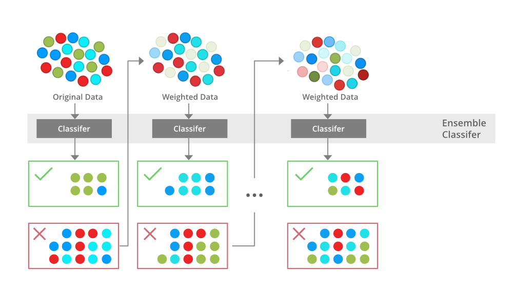
What is AdaBoost

AdaBoost short for Adaptive Boosting is an ensemble learning used in machine learning for classification and regression problems. The main idea behind AdaBoost is to iteratively train the weak classifier on the training dataset with each successive classifier giving more weightage to the data points that are misclassified. The final AdaBoost model is decided by combining all the weak classifier that has been used for training with the weightage given to the models according to their accuracies. The weak model which has the highest accuracy is given the highest weightage while the model which has the lowest accuracy is given a lower weightage. 

Institution Behind AdaBost Algorithm

AdaBoost techniques combine many weak machine-learning models to create a powerful classification model for the output. The steps to build and combine these models are as 

Step1 – Initialize the weights

• For a dataset with N training data points instances, initialize N W_{i} weights for each data point with W_{i} = \frac{1}{N}  

Step2 – Train weak classifiers

• Train a weak classifier M_k where k is the current iteration 
• The weak classifier we are training should have an accuracy greater than 0.5 which means it should be performing better than a naive guess

Step3 – Calculate the error rate and importance of each weak model M_k 

• Calculate rate error_rate for every weak classifier M_k on the training dataset 
• Calculate the importance of each model α_k using formula  \alpha_k = \frac{1}{2} \ln{\frac{1 – error_k}{error_k}}

Step4 – Update data point weight for each data point W_i 

• After applying the weak classifier model to the training data we will update the weight assigned to the points using the accuracy of the model. The formula for updating the weights will be w_i = w_i \exp{(-\alpha_k y_i M_k(x_i))} . Here y_i is the true output and X_i is the corresponding input vector 

Step5 – Normalize the Instance weight 

• We will normalize the instance weight so that they can be summed up to 1 using the formula W_i = W_i / sum(W)

Step6 – Repeat steps 2-5 for K iterations 

• We will train K classifiers and will calculate model importance and update the instance weights using the above formula 
• The final model M(X) will be an ensemble model which is obtained by combining these weak models weighted by their model weights 

Boosting Algorithms 

Python implementation of AdaBoost 

Python provides special packages for applying AdaBoost we will see how we can use Python for applying AdaBoost on a machine learning problem. 

In this problem, we are given a dataset containing 3 species of flowers and the features of these flowers such as sepal length, sepal width, petal length, and petal width, and we have to classify the flowers into these species.

Import Libraries

Let’s begin with importing important libraries that we will require to do our classification task:

Python

import pandas as pd
import numpy as np
from sklearn.model_selection import train_test_split
from sklearn.ensemble import AdaBoostClassifier
import warnings
warnings.filterwarnings("ignore")

Reading  And Describing The Dataset 

 After, importing the libraries we will load our dataset using the pandas read_csv method as:

Python

# Reading the dataset from the csv file
# separator is a vertical line, as seen in the dataset
data = pd.read_csv("Iris.csv")

# Printing the shape of the dataset
print(data.shape)

(150, 6)

We can see our dataset contains 150 rows and 6 columns. Let us take a look at our actual content in the dataset using head() method as:

Python

data.head()

	Id	SepalLengthCm	SepalWidthCm	PetalLengthCm	PetalWidthCm	Species
0	1	5.1	3.5	1.4	0.2	Iris-setosa
1	2	4.9	3.0	1.4	0.2	Iris-setosa
2	3	4.7	3.2	1.3	0.2	Iris-setosa
3	4	4.6	3.1	1.5	0.2	Iris-setosa
4	5	5.0	3.6	1.4	0.2	Iris-setosa

Dropping Irrevelant Column and Separating Target Variable 

The first column is the Id column which has no relevance to flowers so, we will drop it using drop() function. The Species column is our target feature and tells us about the species the flowers belong to. We will separate it using pandas iloc slicing.

Python

data = data.drop('Id',axis=1)
X = data.iloc[:,:-1]
y = data.iloc[:,-1]
print("Shape of X is %s and shape of y is %s"%(X.shape,y.shape))

Shape of X is (150, 4) and shape of y is (150,)

Unique values in our Target Variable 

Since this is a classification task we will see the numbers of categories we want to classify our dataset input vector into. 

Python

total_classes = y.nunique()
print("Number of unique species in dataset are: ",total_classes)

Number of unique species in dataset are: 3

Python

distribution = y.value_counts()
print(distribution)

Iris-virginica     50
Iris-setosa        50
Iris-versicolor    50
Name: Species, dtype: int64

Let’s dig deep into our dataset, and we can see in the above image that our dataset contains 3 classes into which our flowers are distributed also since we have 150 samples all three species have an equal number of samples in the dataset, so we have no class imbalance.

Splitting The Dataset 

Now, we will split the dataset for training and validation purposes, the validation set is 25% of the total dataset. For dividing the dataset into training and testing we will use train_test_split method from the sklearn model selection.  

Python

X_train, X_val, Y_train, Y_val = train_test_split(
    X, y, test_size=0.25, random_state=28)

Applying AdaBoost

After creating the training and validation set we will build our AdaBoost classifier model and fit it over the training set for learning. To fit our AdaBoost model we need our dependent variable y and independent variable x. 

Python

# Creating adaboost classifier model
adb = AdaBoostClassifier()
adb_model = adb.fit(X_train,Y_train)

Accuracy of the AdaBoost Model 

As we fit our model on the train set, we will check the accuracy of our model on the validation set. To check the accuracy of the model we will use the validation dataset that we have created using the train_test_split method. 

Python

print("The accuracy of the model on validation set is", adb_model.score(X_val,Y_val))

The accuracy of the model on validation set is 0.9210526315789473

As we can see the model has an accuracy of 92% on the validation set which is quite good with no hyperparameter tuning and feature engineering.