In statistics, various tests are used to compare different samples or groups and draw conclusions about populations. These tests, known as statistical tests, focus on analyzing the likelihood or probability of obtaining the observed data under specific assumptions or hypotheses. They provide a framework for assessing evidence in support of or against a particular hypothesis.
A statistical test begins by formulating a null hypothesis (H0) and an alternative hypothesis (Ha). The null hypothesis represents the default assumption, typically stating no effect or no difference, while the alternative hypothesis suggests a specific relationship or effect.
There are different statistical tests like Z-test, T-test, Chi-squared tests, ANOVA, Z-test, and F-test, etc. which are used to compute the p-value. In this article, we will learn about the T-test.
What is T-Test?
The t-test is named after William Sealy Gosset’s Student’s t-distribution, created while he was writing under the pen name “Student.”
A t-test is a type of inferential statistic test used to determine if there is a significant difference between the means of two groups. It is often used when data is normally distributed and population variance is unknown.
The t-test is used in hypothesis testing to assess whether the observed difference between the means of the two groups is statistically significant or just due to random variation.
Assumptions in T-test
- Independence: The observations within each group must be independent of each other. This means that the value of one observation should not influence the value of another observation. Violations of independence can occur with repeated measures, paired data, or clustered data.
- Normality: The data within each group should be approximately normally distributed i.e the distribution of the data within each group being compared should resemble a normal (bell-shaped) distribution. This assumption is crucial for small sample sizes (n < 30).
- Homogeneity of Variances (for independent samples t-test): The variances of the two groups being compared should be equal. This assumption ensures that the groups have a similar spread of values. Unequal variances can affect the standard error of the difference between means and, consequently, the t-statistic.
- Absence of Outliers: There should be no extreme outliers in the data as outliers can disproportionately influence the results, especially when sample sizes are small.
Prerequisites for T-Test
Let’s quickly review some related terms before digging deeper into the specifics of the t-test.
A t-test is a statistical method used to compare the means of two groups to determine if there is a significant difference between them. The t-test is a parametric test, meaning it makes certain assumptions about the data. Here are the key prerequisites for conducting a t-test.
Hypothesis Testing:
Hypothesis testing is a statistical method used to make inferences about a population based on a sample of data.
P-value:
The p-value is the probability of observing a test statistic (or something more extreme) given that the null hypothesis is true.
- A small p-value (typically less than the chosen significance level) suggests that the observed data is unlikely to have occurred by random chance alone, leading to the rejection of the null hypothesis.
- A large p-value suggests that the observed data is likely to have occurred by random chance, and there is not enough evidence to reject the null hypothesis.
Degree of freedom (df):
The degree of freedom represents the number of values in a calculation that is free to vary. The degree of freedom (df) tells us the number of independent variables used for calculating the estimate between 2 sample groups.
In a t-test, the degree of freedom is calculated as the total sample size minus 1 i.e  , where “ns” is the number of observations in the sample. It reflects the number of values in the sample that are free to vary after estimating the sample mean.
Suppose, we have 2 samples A and B. The df would be calculated as 
Significance Level:
The significance level is the predetermined threshold that is used to decide whether to reject the null hypothesis. Commonly used significance levels are 0.05, 0.01, or 0.10.
A significance level of 0.05 indicates that the researcher is willing to accept a 5% chance of making a Type I error (incorrectly rejecting a true null hypothesis).
T-statistic:
The t-statistic is a measure of the difference between the means of two groups relative to the variability within each group. It is calculated as the difference between the sample means divided by the standard error of the difference. It is also known as the t-value or t-score.
- If the t-value is large => the two groups belong to different groups.
- If the t-value is small => the two groups belong to the same group.
T-Distribution
The t-distribution, commonly known as the Student’s t-distribution, is a probability distribution with tails that are thicker than those of the normal distribution.
Statistical Significance
Statistical significance is determined by comparing the p-value to the chosen significance level.
- If the p-value is less than or equal to the significance level, the result is considered statistically significant, and the null hypothesis is rejected.
- If the p-value is greater than the significance level, the result is not statistically significant, and there is insufficient evidence to reject the null hypothesis.
In the context of a t-test, these concepts are applied to compare means between two groups. The t-test assesses whether the means are significantly different from each other, taking into account the variability within the groups. The p-value from the t-test is then compared to the significance level to make a decision about the null hypothesis.
A t-table, or a t-distribution table, is a reference table that provides critical values for the t-test. The table is organized by degrees of freedom and significance levels (usually 0.05 or 0.01). The t-table is used to find the critical t-value corresponding to their specific degrees of freedom and chosen significance level. If the calculated t-value is greater than the critical value from the table, it suggests that the observed difference is statistically significant.
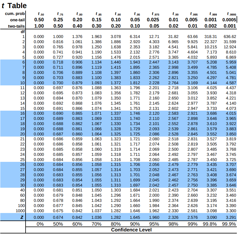
T-Table
Types of T-tests
There are three types of t-tests, and they are categorized as dependent and independent t-tests.
- One sample t-test test: The mean of a single group against a known mean.
- Two-sample t-test: It is further divided into two types:
- Independent samples t-test: compares the means for two groups.
- Paired sample t-test: compares means from the same group at different times (say, one year apart).
One sample T-test
One sample t-test is one of the widely used t-tests for comparison of the sample mean of the data to a particularly given value. Used for comparing the sample mean to the true/population mean.
We can use this when the sample size is small. (under 30) data is collected randomly and it is approximately normally distributed. It can be calculated as:

where,
- t = t-value
- x_bar = sample mean
- μ = true/population mean
- σ = standard deviation
- n = sample size
Example Problem
Consider the following example. The weights of 25 obese people were taken before enrolling them into the nutrition camp. The population mean weight is found to be 45 kg before starting the camp. After finishing the camp, for the same 25 people, the sample mean was found to be 75 with a standard deviation of 25. Did the fitness camp work?
One-Sample T-test in Python
Python3
import scipy.stats as stats
import numpy as np
population_mean = 45
sample_mean = 75
sample_std = 25
sample_size = 25
t_statistic = (sample_mean - population_mean) / (sample_std / np.sqrt(sample_size))
df = sample_size - 1
alpha = 0.05
critical_t = stats.t.ppf(1 - alpha, df)
p_value = 1 - stats.t.cdf(t_statistic, df)
print("T-Statistic:", t_statistic)
print("Critical t-value:", critical_t)
print("P-Value:", p_value)
print('With T-value :')
if t_statistic > critical_t:
print(
)
else:
print(
)
print('With P-value :')
if p_value >alpha:
print(
)
else:
print(
)
|
Output:
T-Statistic: 6.0
Critical t-value: 1.7108820799094275
P-Value: 1.703654035845048e-06
With T-value :
There is a significant difference in weight before and after the camp.
    The fitness camp had an effect.
With P-value :
There is no significant difference in weight before and after the camp.
    The fitness camp did not have a significant effect.
The T-value of 6.0 is significantly greater than the critical t-value, leading to rejection of the null hypothesis therefore, we can conclude there is a significant difference in weight before and after the fitness camp. The fitness camp had an effect on the weights of the participants.
The results strongly suggest that the fitness camp was effective in producing a statistically significant change in weight for the participants.
- The T-value and p-value both provide consistent evidence for rejecting the null hypothesis.
- The practical significance should also be considered to understand the real-world impact of this weight change.
Independent sample T-test
An Independent sample t-test, commonly known as an unpaired sample t-test is used to find out if the differences found between two groups is actually significant or just a random occurrence.
We can use this when:
- the population mean or standard deviation is unknown. (information about the population is unknown)
- the two samples are separate/independent. For eg. boys and girls (the two are independent of each other)
It can be calculated using:

Where,
 are the means of the two groups.
 are the standard deviations of the two groups.
 are the sample sizes of the two groups.
Example Problem
Researchers are investigating whether there is a significant difference in the exam scores of two different teaching methods, A and B. Two independent samples, each representing a different teaching method, have been collected. The objective is to determine if there is enough evidence to suggest that one teaching method leads to higher exam scores compared to the other. Suppose, two independent sample data A and B are given, with the following values. We have to perform the Independent samples t-test for this data.
Sample A (Teaching Method A): 78,84,92,88,75,80,85,90,87,7978,84,92,88,75,80,85,90,87,79
Sample B (Teaching Method B): 82,88,75,90,78,85,88,77,92,8082,88,75,90,78,85,88,77,92,80
Two-Sample t-test in Python (Independent)
Python3
from scipy import stats
import numpy as np
sample_A = np.array([78,84,92,88,75,80,85,90,87,7978,84,92,88,75,80,85,90,87,79])
sample_B = np.array([82,88,75,90,78,85,88,77,92,8082,88,75,90,78,85,88,77,92,80])
t_statistic, p_value = stats.ttest_ind(sample_A, sample_B)
alpha = 0.05
df = len(sample_A)+len(sample_B)-2
critical_t = stats.t.ppf(1 - alpha/2, df)
print("T-value:", t_statistic)
print("P-Value:", p_value)
print("Critical t-value:", critical_t)
print('With T-value')
if np.abs(t_statistic) >critical_t:
print('There is significant difference between two groups')
else:
print('No significant difference found between two groups')
print('With P-value')
if p_value >alpha:
print('No evidence to reject the null hypothesis that a significant difference between the two groups')
else:
print('Evidence found to reject the null hypothesis that a significant difference between the two groups')
|
Output:
T-value: 0.9890707100936805
P-Value: 0.33573862223613105
Critical t-value: 2.10092204024096
With T-value
No significant difference found between two groups
With P-value
No evidence to reject the null hypothesis that a significant difference between the two groups
With T-Value, of 0.989 is less than the critical t-value of 2.1009. Therefore, No significant difference is found between the exam scores of Teaching Method A and Teaching Method B based on the T-value.
With P-Value, of 0.336 is greater than the significance level of 0.05. There is no evidence to reject the null hypothesis, indicating no significant difference between the two teaching methods based on the P-value.
In conclusion, The results suggest that, statistically, there is no significant difference in exam scores between Teaching Method A and Teaching Method B. Therefore, based on this analysis, there is no clear evidence to suggest that one teaching method leads to higher exam scores compared to the other.
Paired Two-sample T-test
Paired sample t-test, commonly known as dependent sample t-test is used to find out if the difference in the mean of two samples is 0. The test is done on dependent samples, usually focusing on a particular group of people or things. In this, each entity is measured twice, resulting in a pair of observations.
We can use this when:
- Two similar (twin like) samples are given. [Eg, Scores obtained in English and Math (both subjects)]
- The dependent variable (data) is continuous.
- The observations are independent of one another.
- The dependent variable is approximately normally distributed.
It can be calculated using,

where,
 is the mean of the differences between the paired observations.
- (s_d) is the standard deviation of the differences.
- (n) is the number of paired observations.
Example Problem
Consider the following example. Scores (out of 25) of the subjects Math1 and Math2 are taken for a sample of 10 students. We have to perform the paired sample t-test for this data.
Math1: 4, 4, 7, 16, 20, 11, 13, 9, 11, 15
Math2:15, 16, 14, 14, 22, 22, 23, 18, 18, 19
Paired Two-Sample T-test in Python
Python3
from scipy import stats
import numpy as np
math1 = np.array([4, 4, 7, 16, 20, 11, 13, 9, 11, 15])
math2 = np.array([15, 16, 14, 14, 22, 22, 23, 18, 18, 19])
t_statistic, p_value = stats.ttest_rel(math1, math2)
alpha = 0.05
df = len(math2)-1
critical_t = stats.t.ppf(1 - alpha/2, df)
print("T-value:", t_statistic)
print("P-Value:", p_value)
print("Critical t-value:", critical_t)
print('With T-value')
if np.abs(t_statistic) >critical_t:
print('There is significant difference between math1 and math2')
else:
print('No significant difference found between math1 and math2')
print('With P-value')
if p_value >alpha:
print('No evidence to reject the null hypothesis that significant difference between math1 and math2')
else:
print('Evidence found to reject the null hypothesis that significant difference between math1 and math2')
|
Output:
T-value: -4.953488372093023
P-Value: 0.0007875235561560145
Critical t-value: 2.2621571627409915
With T-value
There is significant difference between math1 and math2
With P-value
Evidence found to reject the null hypothesis that significant difference between math1 and math2
The paired sample t-test suggests that there is a statistically significant difference in scores between Math1 and Math2 as T-value of -4.95 is less than the critical t-value of -2.2622 and P-value of 0.00079 is less than the significance level of 0.05. Therefore, based on this analysis, it can be concluded that there is evidence to support the claim that the two sets of scores are different, and the difference is not due to random chance.
The above-discussed types of t-tests are widely used in the fields of research in hospitals by experts to gain important information about the medical data given to them about the effects of various medicines and drugs on the population and help them draw out important inferences regarding the same. However, it is the responsibility of the person to see to it that which t-test would bring out the best results and that all the assumptions of that t-test are adhered to. For any doubt/query, comment below.
Conclusion
In conclusion, t-test, play a crucial role in hypothesis testing, comparing means, and drawing conclusions about populations. The test can be one-sample, independent two-sample, or paired two-sample, each with specific use cases and assumptions. Interpretation of results involves considering T-values, P-values, and critical values.
These tests aid researchers in making informed decisions based on statistical evidence.
Frequently Asked Questions on T-Test
Q. What is the t-test for mean in Python?
The t-test for mean in Python is a statistical method used to determine if there is a significant difference between the means of two groups.
Q. What is the t-test function?
The t-test function is a statistical tool used to compare means and assess the significance of differences between groups, considering factors like sample size and variability.
Q. What is the p-value in t-test Python?
The p-value in a t-test Python indicates the probability of observing the data or more extreme results assuming the null hypothesis is true. A small p-value suggests evidence against the null hypothesis.
Q. Why is it called t-test?
The t-test is named after William Sealy Gosset, who published under the pseudonym “Student.” The name “t” refers to the t-distribution used in the test, particularly applicable for small sample sizes.
Share your thoughts in the comments
Please Login to comment...