Decision Tree is one of the most powerful and popular algorithms. Python Decision-tree algorithm falls under the category of supervised learning algorithms. It works for both continuous as well as categorical output variables. In this article, We are going to implement a Decision tree in Python algorithm on the Balance Scale Weight & Distance Database presented on the UCI.
Decision Tree
A Decision tree is a tree-like structure that represents a set of decisions and their possible consequences. Each node in the tree represents a decision, and each branch represents an outcome of that decision. The leaves of the tree represent the final decisions or predictions.
Decision trees are created by recursively partitioning the data into smaller and smaller subsets. At each partition, the data is split based on a specific feature, and the split is made in a way that maximizes the information gain.
Decision Tree
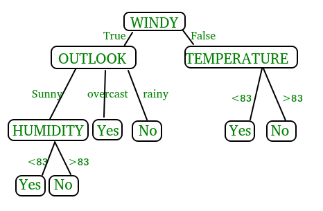
In the above figure, decision tree is a flowchart-like tree structure that is used to make decisions. It consists of Root Node(WINDY), Internal nodes(OUTLOOK, TEMPERATURE), which represent tests on attributes, and leaf nodes, which represent the final decisions. The branches of the tree represent the possible outcomes of the tests.
Key Components of Decision Trees in Python
- Root Node: The decision tree’s starting node, which stands for the complete dataset.
- Branch Nodes: Internal nodes that represent decision points, where the data is split based on a specific attribute.
- Leaf Nodes: Final categorization or prediction-representing terminal nodes.
- Decision Rules: Rules that govern the splitting of data at each branch node.
- Attribute Selection: The process of choosing the most informative attribute for each split.
- Splitting Criteria: Metrics like information gain, entropy, or the Gini Index are used to calculate the optimal split.
Assumptions we make while using Decision tree
- At the beginning, we consider the whole training set as the root.
- Attributes are assumed to be categorical for information gain and for gini index, attributes are assumed to be continuous.
- On the basis of attribute values records are distributed recursively.
- We use statistical methods for ordering attributes as root or internal node.
Pseudocode of Decision tree
- Find the best attribute and place it on the root node of the tree.
- Now, split the training set of the dataset into subsets. While making the subset make sure that each subset of training dataset should have the same value for an attribute.
- Find leaf nodes in all branches by repeating 1 and 2 on each subset.
Key concept in Decision Tree
Gini index and information gain both of these methods are used to select from the n attributes of the dataset which attribute would be placed at the root node or the internal node.

- Gini Index is a metric to measure how often a randomly chosen element would be incorrectly identified.
- It means an attribute with lower gini index should be preferred.
- Sklearn supports “gini” criteria for Gini Index and by default, it takes “gini” value.
If a random variable x can take N different value, the i’value  with probability
  we can associate the following entropy with x :

- Entropy is the measure of uncertainty of a random variable, it characterizes the impurity of an arbitrary collection of examples. The higher the entropy the more the information content.
Information Gain
Definition: Suppose S is a set of instances, A is an attribute,  is the subset of s with A = v and Values(A) is the set of all possible of A, then
- The entropy typically changes when we use a node in a Python decision tree to partition the training instances into smaller subsets. Information gain is a measure of this change in entropy.
- Sklearn supports “entropy” criteria for Information Gain and if we want to use Information Gain method in sklearn then we have to mention it explicitly.
Python Decision Tree Implementation
Dataset Description:
Title                               : Balance Scale Weight & Distance
Database
Number of Instances  : 625 (49 balanced, 288 left, 288 right)
Number of Attributes  : 4 (numeric) + class name = 5
Attribute Information:
1. Class Name (Target variable): 3
       L [balance scale tip to the left]
       B [balance scale be balanced]
       R [balance scale tip to the right]
2. Left-Weight: 5 (1, 2, 3, 4, 5)
3. Left-Distance: 5 (1, 2, 3, 4, 5)
4. Right-Weight: 5 (1, 2, 3, 4, 5)
5. Right-Distance: 5 (1, 2, 3, 4, 5)
Missing Attribute Values: None
Class Distribution:
      1. 46.08 percent are L
      2. 07.84 percent are B
      3. 46.08 percent are R
You can find more details of the dataset.
Prerequsite
- sklearn :
- In python, sklearn is a machine learning package which include a lot of ML algorithms.
- Here, we are using some of its modules like train_test_split, DecisionTreeClassifier and accuracy_score.
- NumPy :
- It is a numeric python module which provides fast maths functions for calculations.
- It is used to read data in numpy arrays and for manipulation purpose.
- Pandas :
- Used to read and write different files.
- Data manipulation can be done easily with dataframes.
Installation of the packages
In Python, sklearn is the package which contains all the required packages to implement Machine learning algorithm. You can install the sklearn package by following the commands given below.
using pip
pip install -U scikit-learn
Before using the above command make sure you have scipy and numpy packages installed. If you don’t have pip. You can install it using
python get-pip.py
using conda
conda install scikit-learn
While implementing the decision tree in Python we will go through the following two phases:
- Building Phase
- Preprocess the dataset.
- Split the dataset from train and test using Python sklearn package.
- Train the classifier.
- Operational Phase
- Make predictions.
- Calculate the accuracy.
Data Import
- To import and manipulate the data we are using the pandas package provided in python.
- Here, we are using a URL which is directly fetching the dataset from the UCI site no need to download the dataset. When you try to run this code on your system make sure the system should have an active Internet connection.
- As the dataset is separated by “,” so we have to pass the sep parameter’s value as “,”.
- Another thing is notice is that the dataset doesn’t contain the header so we will pass the Header parameter’s value as none. If we will not pass the header parameter then it will consider the first line of the dataset as the header.
Data Slicing
- Before training the model we have to split the dataset into the training and testing dataset.
- To split the dataset for training and testing we are using the sklearn module train_test_split
- First of all we have to separate the target variable from the attributes in the dataset.
X = balance_data.values[:, 1:5]
Y = balance_data.values[:,0]
- Above are the lines from the code which separate the dataset. The variable X contains the attributes while the variable Y contains the target variable of the dataset.
- Next step is to split the dataset for training and testing purpose.
X_train, X_test, y_train, y_test = train_test_split(
          X, Y, test_size = 0.3, random_state = 100)
- Above line split the dataset for training and testing. As we are splitting the dataset in a ratio of 70:30 between training and testing so we are pass test_size parameter’s value as 0.3.
- random_state variable is a pseudo-random number generator state used for random sampling.
Building a Decision Tree in Python
Below is the code for the sklearn decision tree in Python.
Import Library
Importing the necessary libraries required for the implementation of decision tree in Python.
Python3
import numpy as np
import pandas as pd
from sklearn.metrics import confusion_matrix, accuracy_score, classification_report
from sklearn.model_selection import train_test_split
from sklearn.tree import DecisionTreeClassifier
import matplotlib.pyplot as plt
|
Data Import and Exploration
Python3
def importdata():
balance_data = pd.read_csv(
'databases/balance-scale/balance-scale.data',
sep=',', header=None)
print("Dataset Length: ", len(balance_data))
print("Dataset Shape: ", balance_data.shape)
print("Dataset: ", balance_data.head())
return balance_data
|
Data Splitting
splitdataset(balance_data): This function defines the splitdataset() function, which is responsible for splitting the dataset into training and testing sets. It separates the target variable (class labels) from the features and splits the data using the train_test_split() function from scikit-learn. It sets the test size to 30% and uses a random state of 100 for reproducibility.
Python3
def splitdataset(balance_data):
X = balance_data.values[:, 1:5]
Y = balance_data.values[:, 0]
X_train, X_test, y_train, y_test = train_test_split(
X, Y, test_size=0.3, random_state=100)
return X, Y, X_train, X_test, y_train, y_test
|
Training with Gini Index:
train_using_gini(X_train, X_test, y_train): This function defines the train_using_gini() function, which is responsible for training a decision tree classifier using the Gini index as the splitting criterion. It creates a classifier object with the specified parameters (criterion, random state, max depth, min samples leaf) and trains it on the training data.
Python3
def train_using_gini(X_train, X_test, y_train):
clf_gini = DecisionTreeClassifier(criterion="gini",
random_state=100, max_depth=3, min_samples_leaf=5)
clf_gini.fit(X_train, y_train)
return clf_gini
|
Training with Entropy:
tarin_using_entropy(X_train, X_test, y_train): This function defines the tarin_using_entropy() function, which is responsible for training a decision tree classifier using entropy as the splitting criterion. It creates a classifier object with the specified parameters (criterion, random state, max depth, min samples leaf) and trains it on the training data.
Python3
def tarin_using_entropy(X_train, X_test, y_train):
clf_entropy = DecisionTreeClassifier(
criterion="entropy", random_state=100,
max_depth=3, min_samples_leaf=5)
clf_entropy.fit(X_train, y_train)
return clf_entropy
|
Prediction and Evaluation:
prediction(X_test, clf_object): This function defines the prediction() function, which is responsible for making predictions on the test data using the trained classifier object. It passes the test data to the classifier’s predict() method and prints the predicted class labels.cal_accuracy(y_test, y_pred): This function defines the cal_accuracy() function, which is responsible for calculating the accuracy of the predictions. It calculates and prints the confusion matrix, accuracy score, and classification report, providing detailed performance evaluation.
Python3
def prediction(X_test, clf_object):
y_pred = clf_object.predict(X_test)
print("Predicted values:")
print(y_pred)
return y_pred
def cal_accuracy(y_test, y_pred):
print("Confusion Matrix: ",
confusion_matrix(y_test, y_pred))
print("Accuracy : ",
accuracy_score(y_test, y_pred)*100)
print("Report : ",
classification_report(y_test, y_pred))
|
Plots the Decision Tree
By using plot_tree function from the sklearn.tree submodule to plot the decision tree. The function takes the following arguments:
clf_object: The trained decision tree model object.filled=True: This argument fills the nodes of the tree with different colors based on the predicted class majority.feature_names: This argument provides the names of the features used in the decision tree.class_names: This argument provides the names of the different classes.rounded=True: This argument rounds the corners of the nodes for a more aesthetically pleasing appearance.
Python3
def plot_decision_tree(clf_object, feature_names, class_names):
plt.figure(figsize=(15, 10))
plot_tree(clf_object, filled=True, feature_names=feature_names, class_names=class_names, rounded=True)
plt.show()
|
This defines two decision tree classifiers, training and visualization of decision trees based on different splitting criteria, one using the Gini index and the other using entropy,
Python3
if __name__ == "__main__":
data = importdata()
X, Y, X_train, X_test, y_train, y_test = splitdataset(data)
clf_gini = train_using_gini(X_train, X_test, y_train)
clf_entropy = train_using_entropy(X_train, X_test, y_train)
plot_decision_tree(clf_gini, ['X1', 'X2', 'X3', 'X4'], ['L', 'B', 'R'])
plot_decision_tree(clf_entropy, ['X1', 'X2', 'X3', 'X4'], ['L', 'B', 'R'])
|
Output:
DATA INFO
Dataset Length:  625
Dataset Shape:  (625, 5)
Dataset:     0  1  2  3  4
0  B  1  1  1  1
1  R  1  1  1  2
2  R  1  1  1  3
3  R  1  1  1  4
4  R  1  1  1  5
Using Gini Index
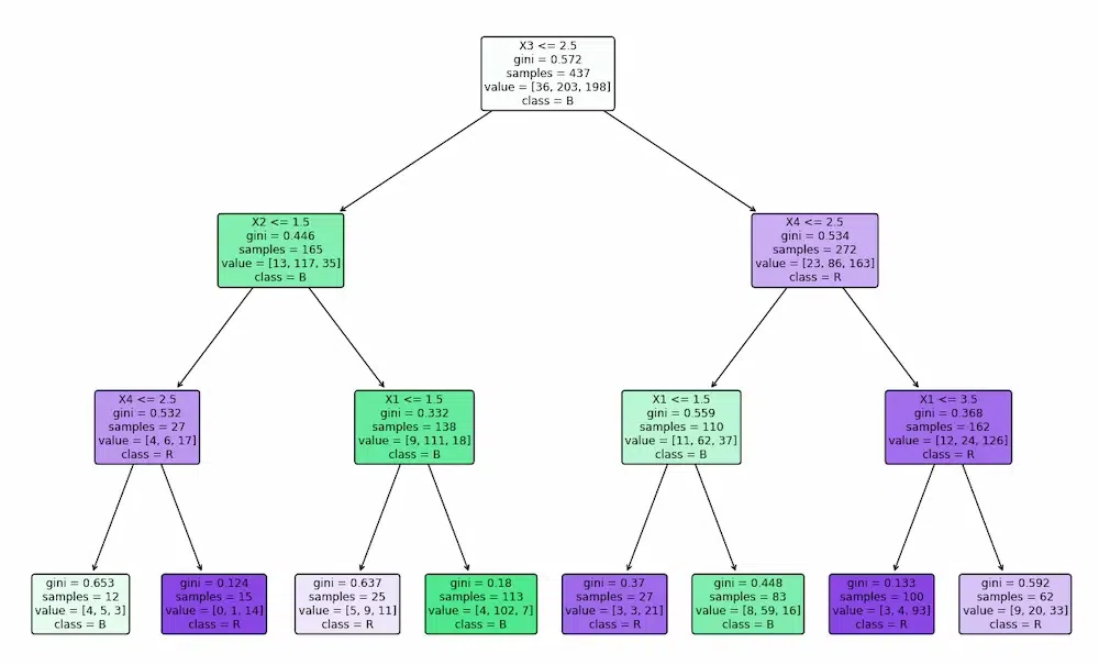
Using Entropy
.webp)
It performs the operational phase of the decision tree model, which involves:
- Imports and splits data for training and testing.
- Uses Gini and entropy criteria to train two decision trees.
- Generates class labels for test data using each model.
- Calculates and compares accuracy of both models.
Evaluates the performance of the trained decision trees on the unseen test data and provides insights into their effectiveness for the specific classification task and evaluates their performance on a dataset using the confusion matrix, accuracy score, and classification report.
Results using Gini Index
Python3
print("Results Using Gini Index:")
y_pred_gini = prediction(X_test, clf_gini)
cal_accuracy(y_test, y_pred_gini)
|
Output:
Results Using Gini Index:
Predicted values:
['R' 'L' 'R' 'R' 'R' 'L' 'R' 'L' 'L' 'L' 'R' 'L' 'L' 'L' 'R' 'L' 'R' 'L'
 'L' 'R' 'L' 'R' 'L' 'L' 'R' 'L' 'L' 'L' 'R' 'L' 'L' 'L' 'R' 'L' 'L' 'L'
 'L' 'R' 'L' 'L' 'R' 'L' 'R' 'L' 'R' 'R' 'L' 'L' 'R' 'L' 'R' 'R' 'L' 'R'
 'R' 'L' 'R' 'R' 'L' 'L' 'R' 'R' 'L' 'L' 'L' 'L' 'L' 'R' 'R' 'L' 'L' 'R'
 'R' 'L' 'R' 'L' 'R' 'R' 'R' 'L' 'R' 'L' 'L' 'L' 'L' 'R' 'R' 'L' 'R' 'L'
 'R' 'R' 'L' 'L' 'L' 'R' 'R' 'L' 'L' 'L' 'R' 'L' 'R' 'R' 'R' 'R' 'R' 'R'
 'R' 'L' 'R' 'L' 'R' 'R' 'L' 'R' 'R' 'R' 'R' 'R' 'L' 'R' 'L' 'L' 'L' 'L'
 'L' 'L' 'L' 'R' 'R' 'R' 'R' 'L' 'R' 'R' 'R' 'L' 'L' 'R' 'L' 'R' 'L' 'R'
 'L' 'L' 'R' 'L' 'L' 'R' 'L' 'R' 'L' 'R' 'R' 'R' 'L' 'R' 'R' 'R' 'R' 'R'
 'L' 'L' 'R' 'R' 'R' 'R' 'L' 'R' 'R' 'R' 'L' 'R' 'L' 'L' 'L' 'L' 'R' 'R'
 'L' 'R' 'R' 'L' 'L' 'R' 'R' 'R']
Confusion Matrix:  [[ 0  6  7]
 [ 0 67 18]
 [ 0 19 71]]
Accuracy :  73.40425531914893
Report :                precision    recall  f1-score   support
           B       0.00      0.00      0.00        13
           L       0.73      0.79      0.76        85
           R       0.74      0.79      0.76        90
    accuracy                           0.73       188
   macro avg       0.49      0.53      0.51       188
weighted avg       0.68      0.73      0.71       188
Results using Entropy
Python3
print("Results Using Entropy:")
y_pred_entropy = prediction(X_test, clf_entropy)
cal_accuracy(y_test, y_pred_entropy)
|
Output:
Results Using Entropy:
Predicted values:
['R' 'L' 'R' 'L' 'R' 'L' 'R' 'L' 'R' 'R' 'R' 'R' 'L' 'L' 'R' 'L' 'R' 'L'
 'L' 'R' 'L' 'R' 'L' 'L' 'R' 'L' 'R' 'L' 'R' 'L' 'R' 'L' 'R' 'L' 'L' 'L'
 'L' 'L' 'R' 'L' 'R' 'L' 'R' 'L' 'R' 'R' 'L' 'L' 'R' 'L' 'L' 'R' 'L' 'L'
 'R' 'L' 'R' 'R' 'L' 'R' 'R' 'R' 'L' 'L' 'R' 'L' 'L' 'R' 'L' 'L' 'L' 'R'
 'R' 'L' 'R' 'L' 'R' 'R' 'R' 'L' 'R' 'L' 'L' 'L' 'L' 'R' 'R' 'L' 'R' 'L'
 'R' 'R' 'L' 'L' 'L' 'R' 'R' 'L' 'L' 'L' 'R' 'L' 'L' 'R' 'R' 'R' 'R' 'R'
 'R' 'L' 'R' 'L' 'R' 'R' 'L' 'R' 'R' 'L' 'R' 'R' 'L' 'R' 'R' 'R' 'L' 'L'
 'L' 'L' 'L' 'R' 'R' 'R' 'R' 'L' 'R' 'R' 'R' 'L' 'L' 'R' 'L' 'R' 'L' 'R'
 'L' 'R' 'R' 'L' 'L' 'R' 'L' 'R' 'R' 'R' 'R' 'R' 'L' 'R' 'R' 'R' 'R' 'R'
 'R' 'L' 'R' 'L' 'R' 'R' 'L' 'R' 'L' 'R' 'L' 'R' 'L' 'L' 'L' 'L' 'L' 'R'
 'R' 'R' 'L' 'L' 'L' 'R' 'R' 'R']
Confusion Matrix:  [[ 0  6  7]
 [ 0 63 22]
 [ 0 20 70]]
Accuracy :  70.74468085106383
Report :                precision    recall  f1-score   support

           B       0.00      0.00      0.00        13
           L       0.71      0.74      0.72        85
           R       0.71      0.78      0.74        90

    accuracy                           0.71       188
   macro avg       0.47      0.51      0.49       188
weighted avg       0.66      0.71      0.68       188
Applications of Decision Trees
Python Decision trees are versatile tools with a wide range of applications in machine learning:
- Classification: Making predictions about categorical results, like if an email is spam or not.
- Regression: The estimation of continuous values; for example, feature-based home price prediction.
- Feature Selection: Feature selection lowers dimensionality and boosts model performance by determining which features are most pertinent to a certain job.
Conclusion
Python decision trees provide a strong and comprehensible method for handling machine learning tasks. They are an invaluable tool for a variety of applications because of their ease of use, efficiency, and capacity to handle both numerical and categorical data. Decision trees are a useful tool for making precise forecasts and insightful analysis when used carefully.
Frequently Asked Questions(FAQs)
1. What are decision trees?
Decision trees are a type of machine learning algorithm that can be used for both classification and regression tasks. They work by partitioning the data into smaller and smaller subsets based on certain criteria. The final decision is made by following the path through the tree that is most likely to lead to the correct outcome.
2. How do decision trees work?
Decision trees work by recursively partitioning the data into smaller subsets. At each partition, a decision is made based on a certain criterion, such as the value of a particular feature. The data is then partitioned again based on the value of a different feature, and so on. This process continues until the data is divided into a number of subsets that are each relatively homogeneous.
3. How do you implement a decision tree in Python?
There are several libraries available for implementing decision trees in Python. One popular library is scikit-learn. To implement a decision tree in scikit-learn, you can use the DecisionTreeClassifier class. This class has several parameters that you can set, such as the criterion for splitting the data and the maximum depth of the tree.
4. How do you evaluate the performance of a decision tree?
There are several metrics that you can use to evaluate the performance of a decision tree. One common metric is accuracy, which is the proportion of predictions that the tree makes correctly. Another common metric is precision, which is the proportion of positive predictions that are actually correct. And another common metric is recall, which is the proportion of actual positives that the tree correctly identifies as positive.
5. What are some of the challenges of using decision trees?
Some of the challenges of using decision trees include:
- Overfitting: Decision trees can be prone to overfitting, which means that they can learn the training data too well and not generalize well to new data.
- Interpretability: Decision trees can be difficult to interpret when they are very deep or complex.
- Feature selection: Decision trees can be sensitive to the choice of features.
- Pruning: Decision trees can be difficult to prune, which means that it can be difficult to remove irrelevant branches from the tree.
Share your thoughts in the comments
Please Login to comment...